Motivation 🔗
The deep learning classes I’ve taken have all followed a similar progression:
- First, you learn to do the math by hand, using symbols (the input vector is \(x\), the weight matrix is \(W\), \(z = Wx + b\), etc.)
- Next, you write code to implement the math numerically (manipulating arrays or tensors of numbers). At this stage, you write it from scratch using just NumPy arrays.
- Finally, you graduate to writing code that uses deep learning frameworks like TensorFlow and PyTorch.
Step 1 teaches you the theory, and step 3 teaches you the tools that real practitioners use. Step 2 in between teaches you what those tools are doing so you don’t approach them as black boxes. I’m a fan.
I recently took a class on Convolutional Neural Networks. While it followed this progression, it didn’t teach the math for back propagation through convolutional layers. I tried to work this out for myself and found that the math wasn’t hard, but it was tedious (long expressions, lots of superscripts and subscripts to keep track of).
In trying to explore ways to automate some of the tedious parts, I think I found an approach that re-organizes things so that step 2 (writing the code from scratch) borrows an idea from step 3 (automatic differentiation) and as a result, actually helps with step 1 (understanding the math).
Automatic Differentiation as a Convenience 🔗
In the usual progression, the big change between steps 2 and 3 is that the deep learning frameworks give you automatic differentiation capabilities (GradientTape in TensorFlow, autograd in PyTorch). When you write a neural network from scratch, you write the forward and backward passes as separate algorithms that share some data. With auto differentiation, you to write just the forward pass logic and you get the backward pass for free. The framework keeps track of the operations performed in the forward pass and can calculate the partial derivatives required for back propagation automatically.
Auto differentiation reduces the amount of code you need to write to implement a neural network but it isn’t a learning tool. It does its job numerically: given the numerical value of the gradient at some node in a computation graph, you can get the numerical value of the gradient at earlier nodes, but you can’t see the derivatives expressed symbolically. You get the answer but the framework doesn’t show its work. ML Classes introduce auto differentiation frameworks late in the curriculum because they’re a convenience you earn the right to use after you’ve worked through the math the hard way.
Automatic Differentiation as a Learning Tool 🔗
I found a hybrid approach: implementing algorithms from scratch but using a symbolic framework that can auto differentiate while showing its work. It really helped me with my task of deriving the backprop equations for convolutions. This technique isn’t a replacement for doing math by hand and I wouldn’t blindly trust it, but it helped me learn. It automated the math that’s easy - but tedious - to work through by hand, and helped me visualize the patterns behind the equations.
I’ll walk you through what I did. All of the code for this is available on my GitHub.
Convolutions from Scratch 🔗
After the CNN course I took covered the basic math, the first coding exercise was to implement the convolution operation from scratch, using just NumPy (step 2 in the progression I mentioned earlier). Below is the convolution* function I implemented. It’s probably not the most efficient implementation, but writing it was a good learning exercise.
*I’m aware that, mathematically speaking, what I’m implementing here is actually cross-correlation rather than convolution. This article offers a good description of the differences. tl;dr: in true mathematical convolution, you’re supposed to flip the kernel 180° before applying it. But in deep learning, the kernel weights are learned during training so the orientation is not meaningful. Deep-learning practitioners don’t seem to worry about the distinction between convolution and cross-correlation, so I’m going with it.
def convolve(X: np.ndarray, filter: np.ndarray, zero_pad_width: int, stride: int):
    X_pad = np.pad(
        X,
        ((zero_pad_width, zero_pad_width), (zero_pad_width, zero_pad_width)),
        mode='constant',
        constant_values=(0.0, 0.0),
    )

    in_H, in_W = X.shape
    f, f = filter.shape

    out_H = int((in_H + (2 * zero_pad_width) - f) / stride) + 1
    out_W = int((in_W + (2 * zero_pad_width) - f) / stride) + 1

    output = np.zeros((out_H, out_W), dtype=X.dtype)

    for out_row in range(out_H):
        for out_col in range(out_W):
            in_start_row = out_row * stride
            in_start_col = out_col * stride
            output[out_row][out_col] = sum(
                (
                    X_pad[in_row][in_col] * filter[i][j]
                    for i, in_row in enumerate(range(in_start_row, in_start_row + f))
                    for j, in_col in enumerate(range(in_start_col, in_start_col + f))
                )
            )

    return output
We can test it with some sample data:
X_test = np.array(
    [
        [1.0, 2.0, 3.0, 4.0,],
        [1.0, 2.0, 3.0, 4.0,],
        [1.0, 2.0, 3.0, 4.0,],
        [1.0, 2.0, 3.0, 4.0,],
    ]
)


f_test = np.array(
    [
        [0.0, 1.0,],
        [1.0, 0.0,],
    ]
)

expected = np.array(
    [
        [3.0, 5.0, 7.0],
        [3.0, 5.0, 7.0],
        [3.0, 5.0, 7.0]
    ]
)

test_eq(convolve(X_test, f_test, 0, 1), expected)
And it also happens to give the same answer as SciPy’s convolve2d() function!
# Test output of our convolve function is consistent with scipy
test_eq(
    convolve(X_test, f_test, 0, 1), # ours
    convolve2d(X_test, f_test, mode='valid') # scipy
)
So we can be reasonably sure it works.
Numeric vs Symbolic Computing 🔗
In the examples above, the convolution function is a numeric algorithm: it takes numbers as inputs and produces numbers as output. This is exactly what we’d want when building a neural network that we’d actually train and use.
In contrast to numerical algorithms, symbolic computing involves manipulating expressions made of symbols rather than just numbers. SymPy is an open-source symbolic expression library for Python. It lets programs express and manipulate symbolic mathematical expressions. For example:
x = Symbol('x')

expr = 2*x + 3

# expr now contains the expression 2x + 3
expr
\(\displaystyle 2 x + 3\)
SymPy implements a lot of basic math: core operators, simplification, expansion etc. A few more examples:
# Simplification 2x + 4x = 6x:
expr = 2*x + 4*x
print("2x + 4x = ")
display(expr)

# Simplification (2x + 3) - (x + 1) = x + 2
expr1 = 2*x + 3
expr2 = x + 1
print("(2x + 3) - (x + 1) = ")
display(expr1 - expr2)
2x + 4x =
\(\displaystyle 6 x\)
(2x + 3) - (x + 1) =
\(\displaystyle x + 2\)
SymPy can even do calculus, but we’ll look at that in more detail later.
For now, my point is that symbolic computing lets us perform operations and see the expressions that result. This isn’t of any use in a production neural network but it can be a useful learning tool, as I’ll show.
Convolution with Symbols 🔗
It turns out, the same convolution code works just as well when the contents of the input arrays are SymPy symbols instead of numbers:
X_test = np.array([
    [Symbol(r'x_{11}'), Symbol(r'x_{12}'), Symbol(r'x_{13}'), Symbol(r'x_{14}'),],
    [Symbol(r'x_{21}'), Symbol(r'x_{22}'), Symbol(r'x_{23}'), Symbol(r'x_{24}'),],
    [Symbol(r'x_{31}'), Symbol(r'x_{32}'), Symbol(r'x_{33}'), Symbol(r'x_{34}'),],
    [Symbol(r'x_{41}'), Symbol(r'x_{42}'), Symbol(r'x_{43}'), Symbol(r'x_{44}'),],
])


f_test = np.array([
    [Symbol(r'w_{11}'), Symbol(r'w_{12}'),],
    [Symbol(r'w_{21}'), Symbol(r'w_{22}')],
])
result = convolve(X_test, f_test, 0, 1)
result
array([[w_{11}*x_{11} + w_{12}*x_{12} + w_{21}*x_{21} + w_{22}*x_{22},
        w_{11}*x_{12} + w_{12}*x_{13} + w_{21}*x_{22} + w_{22}*x_{23},
        w_{11}*x_{13} + w_{12}*x_{14} + w_{21}*x_{23} + w_{22}*x_{24}],
       [w_{11}*x_{21} + w_{12}*x_{22} + w_{21}*x_{31} + w_{22}*x_{32},
        w_{11}*x_{22} + w_{12}*x_{23} + w_{21}*x_{32} + w_{22}*x_{33},
        w_{11}*x_{23} + w_{12}*x_{24} + w_{21}*x_{33} + w_{22}*x_{34}],
       [w_{11}*x_{31} + w_{12}*x_{32} + w_{21}*x_{41} + w_{22}*x_{42},
        w_{11}*x_{32} + w_{12}*x_{33} + w_{21}*x_{42} + w_{22}*x_{43},
        w_{11}*x_{33} + w_{12}*x_{34} + w_{21}*x_{43} + w_{22}*x_{44}]],
      dtype=object)
Each element of the output array is now an expression in terms of the input symbols that defines how that element is calculated. We can pretty-print the first-one to see it better:
result[0][0]
\(\displaystyle w_{11} x_{11} + w_{12} x_{12} + w_{21} x_{21} + w_{22} x_{22}\)
This is exactly the expression for the first element of the convolution output. If you overlaid the filter on the top-left corner of the input matrix and then multiplied elements and summed the products, this is the expression you’d get. A little helper function will make it easier to see the whole matrix of expressions:
Markdown(matrix_to_markdown(result))
$$\begin{bmatrix} w_{11} x_{11} + w_{12} x_{12} + w_{21} x_{21} + w_{22} x_{22} & w_{11} x_{12} + w_{12} x_{13} + w_{21} x_{22} + w_{22} x_{23} & w_{11} x_{13} + w_{12} x_{14} + w_{21} x_{23} + w_{22} x_{24}\\ w_{11} x_{21} + w_{12} x_{22} + w_{21} x_{31} + w_{22} x_{32} & w_{11} x_{22} + w_{12} x_{23} + w_{21} x_{32} + w_{22} x_{33} & w_{11} x_{23} + w_{12} x_{24} + w_{21} x_{33} + w_{22} x_{34}\\ w_{11} x_{31} + w_{12} x_{32} + w_{21} x_{41} + w_{22} x_{42} & w_{11} x_{32} + w_{12} x_{33} + w_{21} x_{42} + w_{22} x_{43} & w_{11} x_{33} + w_{12} x_{34} + w_{21} x_{43} + w_{22} x_{44}\end{bmatrix} $$
Each element of the result matrix contains the expression that computes it from the symbols in the inputs. And we got this by running the same convolution function that originally worked with numbers.
How Does This Work? 🔗
The convolution code uses the * operator on the elements of the input arrays and the calls sum() built-in function (which uses + implicitly) over the products. When input arrays contained numbers, these operations performed the expected numerical operations.
# Simplified version of what convolve() does:
x11 = 1.0
x12 = 2.0
w11 = 0.0
w12 = 1.0
sum([x11*w11, x12*w12])
2.0
SymPy implements all the basic Python math operators (+. -, *, /, and more) on Symbols and other expression types. So when we passed symbols to convolve(), all the multiplying and adding just invoked SymPy’s implementations of those operators, which produce expressions rather than numerical results.
# Simplified version of what convolve() does:
x11 = Symbol(r'x_{11}')
x12 = Symbol(r'x_{12}')
w11 = Symbol(r'w_{11}')
w12 = Symbol(r'w_{12}')
sum([x11*w11, x12*w12])
\(\displaystyle w_{11} x_{11} + w_{12} x_{12}\)
Indexed Objects 🔗
Before continuing, I want to make one improvement to the way we’re creating the matrices of symbols. In the code above, I created each Symbol in the matrices manually. Obviously, a couple of nested for-loops would accomplish this with less typing.
But beyond that, notice that each symbol name contains its row and column index. SymPy actually has support for the concept of an Indexed Object that makes it a little easier to extract the indices later when doing reflection. So I created a helper function that creates arrays of indexed symbols:
def ndarray_of_indexed_base(
    ib: IndexedBase, shape: Tuple[int, int], transform=lambda x: x
) -> np.ndarray:
    rows, cols = shape
    data = [
        [transform(ib[i, j]) for j in range(1, cols + 1)] for i in range(1, rows + 1)
    ]
    return np.array(data, dtype=object)
With this helper, I can create the equivalent of the X_test matrix above with just one line:
X_test = ndarray_of_indexed_base(IndexedBase('x'), (4, 4))
X_test
array([[x[1, 1], x[1, 2], x[1, 3], x[1, 4]],
       [x[2, 1], x[2, 2], x[2, 3], x[2, 4]],
       [x[3, 1], x[3, 2], x[3, 3], x[3, 4]],
       [x[4, 1], x[4, 2], x[4, 3], x[4, 4]]], dtype=object)
The representation looks a little different but it’s essentially still a matrix of symbols. Our helper function can make it more readable:
Markdown(matrix_to_markdown(X_test))
$$\begin{bmatrix} {x}_{1,1} & {x}_{1,2} & {x}_{1,3} & {x}_{1,4}\\ {x}_{2,1} & {x}_{2,2} & {x}_{2,3} & {x}_{2,4}\\ {x}_{3,1} & {x}_{3,2} & {x}_{3,3} & {x}_{3,4}\\ {x}_{4,1} & {x}_{4,2} & {x}_{4,3} & {x}_{4,4}\end{bmatrix} $$
The reason we want to use Indexed Objects for our symbols is that it’s easier to extract the indices and the name of the “base” (the thing being indexed):
# Test accessing the indices (note that we use zero-based indices to access
# the array but the conceptual matrix indices are 1-based.)
test_eq(X_test[0][0].indices, (1, 1))

# Test getting the name of the base.
test_eq(X_test[0][0].base.name, 'x')
The ability to easily pull out the base name and indices of a symbol will come in handy later when we analyze expressions.
Example from a Convolutional Neural Network 🔗
Let’s assume we’ve got a convolutional layer, somewhere in the middle of a CNN. To make things simple, I imagined the second layer of a CNN (\(\mathcal{l} = 2\)) and that I’d be dealing with:
- the activations from the previous layer, \(a^{[1]}\)
- the weights for the convolution kernel in the current layer, \(W^{[2]}\)
- the bias for the current layer, \(b^{[2]}\)
- the output from the convolution operation and adding the bias, \(z^{[2]}\)
The diagram below, as well as diagrams and animations later in this notebook, are created in code, using Manim. The first folded code cell below contains some common drawing functions that will be used throughout. The second one renders the diagram that follows. I won’t be explaining the drawing code in detail and you can safely ignore it.

For simplicity, I’m assuming \(a^{[1]}\) has just one channel, there’s just a single \(W^{[2]}\) filter, and we’re looking at just a single training example. The following few lines of code implement the forward pass calculation of \(z^{[2]}\) for our layer of interest:
a1 = ndarray_of_indexed_base(IndexedBase(r'a^{[1]}'), (6, 6))
W2 = ndarray_of_indexed_base(IndexedBase(r'W^{[2]}'), (3, 3))
b2 = symbols(r'b^{[2]}')
z2 = convolve(a1, W2, 0, 1) + b2
Visualizing Expressions 🔗
We can examine the elements of z2 to see that they represent the expressions we’d expect. E.g., the first element is:
z2[0][0]
\(\displaystyle b^{[2]} + {W^{[2]}}_{1,1} {a^{[1]}}_{1,1} + {W^{[2]}}_{1,2} {a^{[1]}}_{1,2} + {W^{[2]}}_{1,3} {a^{[1]}}_{1,3} + {W^{[2]}}_{2,1} {a^{[1]}}_{2,1} + {W^{[2]}}_{2,2} {a^{[1]}}_{2,2} + {W^{[2]}}_{2,3} {a^{[1]}}_{2,3} + {W^{[2]}}_{3,1} {a^{[1]}}_{3,1} + {W^{[2]}}_{3,2} {a^{[1]}}_{3,2} + {W^{[2]}}_{3,3} {a^{[1]}}_{3,3}\)
This is exactly the sum of the weights multiplied by the corresponding elements in the left corner of the input matrix, plus the bias term. Similarly, the next element of z2 contains the expression for the next convolution output (notice the \(a^{[1]}\) column indices are shifted over by one):
z2[0][1]
\(\displaystyle b^{[2]} + {W^{[2]}}_{1,1} {a^{[1]}}_{1,2} + {W^{[2]}}_{1,2} {a^{[1]}}_{1,3} + {W^{[2]}}_{1,3} {a^{[1]}}_{1,4} + {W^{[2]}}_{2,1} {a^{[1]}}_{2,2} + {W^{[2]}}_{2,2} {a^{[1]}}_{2,3} + {W^{[2]}}_{2,3} {a^{[1]}}_{2,4} + {W^{[2]}}_{3,1} {a^{[1]}}_{3,2} + {W^{[2]}}_{3,2} {a^{[1]}}_{3,3} + {W^{[2]}}_{3,3} {a^{[1]}}_{3,4}\)
If we wanted to visualize this expression, one way to do it would be to draw the three matrices, \(a^{[1]}\), \(W^{[2]}\), and \(z^{[2]}\), and highlight the elements of \(a^{[1]}\) and \(W^{[2]}\) that are multiplied together to produce a given element of \(z^{[2]}\).
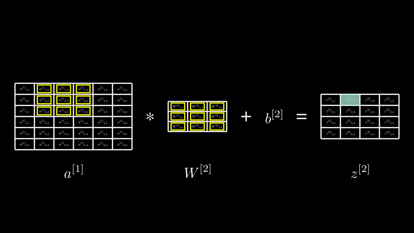
In this visualization and all the others that follow, the “output element” (the element of the convolution result being computed) is highlighted in teal, and the elements of the inputs being multiplied together are outlined in yellow. In the example above, to compute element \(z^{[2]}_{1, 2}\) (highlighted in teal), we multiply the elements of \(W^{[2]}\) with the elements of \(a^{[1]}\) outlined in yellow.
In the code that generated this image, I hardcoded the cells to highlight:
        # Map of cells to highlight
        highlights_map = {
            r'W^{[2]}': [(1, 1), (1, 2), (1, 3), (2, 1), (2, 2), (2, 3), (3, 1), (3, 2), (3, 3)],
            r'a^{[1]}': [(1, 2), (1, 3), (1, 4), (2, 2), (2, 3), (2, 4), (3, 2), (3, 3), (3, 4)],
        }
But we can do better!
Reflecting Over Expressions 🔗
It turns out we can generate this highlights map directly from an expression like:
$$ {W^{[2]}}_{1,1} {a^{[1]}}_{1,2} + {W^{[2]}}_{1,2} {a^{[1]}}_{1,3} + {W^{[2]}}_{1,3} {a^{[1]}}_{1,4} + {W^{[2]}}_{2,1} {a^{[1]}}_{2,2} + {W^{[2]}}_{2,2} {a^{[1]}}_{2,3} + {W^{[2]}}_{2,3} {a^{[1]}}_{2,4} + {W^{[2]}}_{3,1} {a^{[1]}}_{3,2} + {W^{[2]}}_{3,2} {a^{[1]}}_{3,3} + {W^{[2]}}_{3,3} {a^{[1]}}_{3,4} $$
Because that expression is also a data structure. SymPy represents expressions as trees: details are in the documentation but the basic idea is that every expression object has a func attribute and an args attribute that (roughly) correspond to the operator and operands respectively. A few examples:
x = Symbol('x')
expr = 2 + x

# The expressions's `func` is Add
test_eq(expr.func, Add)

# It's `args` are 2 and x
test_eq(expr.args, (2, x))
Using func and args to reflect over expressions, we can write a function that takes an expression and returns a dictionary where the keys are matrix names, and the values are lists of indices to highlight.
def build_highlights_map(expr: Expr) -> Dict[str, List[Tuple]]:
    # The expression needs to be either a sum of products or a single product
    assert expr.func == Add or expr.func == Mul

    # If it's an Add, assert all args are Muls
    if expr.func == Add:
        assert all(arg.func == Mul for arg in expr.args)

    # We want the list of multiplications. This is either a list consisting
    # of just the expression itself if it's a Mul or its arguments if it's
    # an Add.
    muls = [expr] if expr.func == Mul else expr.args

    results = {}
    for expr in muls:
        # Assert all the args are Indexed
        assert all(arg.func == Indexed for arg in expr.args)

        for indexed in expr.args:
            if indexed.base.name not in results:
                results[indexed.base.name] = []
            results[indexed.base.name].append(indexed.indices)
    return results
This function makes a lot of assumptions that it’s dealing with expressions that are just sums of products of Indexed objects, but it suffices for now. We can test it with one of the expressions in the z2 array:
build_highlights_map(z2[0][1]-b2) # Subtract off b2 because we aren't interested in the bias term for now.
{'W^{[2]}': [(1, 1),
  (1, 2),
  (1, 3),
  (2, 1),
  (2, 2),
  (2, 3),
  (3, 1),
  (3, 2),
  (3, 3)],
 'a^{[1]}': [(1, 2),
  (1, 3),
  (1, 4),
  (2, 2),
  (2, 3),
  (2, 4),
  (3, 2),
  (3, 3),
  (3, 4)]}
Animating the Visualization 🔗
Now, we can incorporate that into a Manim scene and add some animation to go through all of the expressions in z2.
This produces a video. To keep the notebook small, I’ve not embedded it directly, but the YouTube version below shows the output. This is a working animation of a convolution, generated directly from the expressions used to compute it.
Other Forms of Convolution 🔗
Because the drawing logic is driven purely off the expressions, it’s trivial to visualize other forms of the convolution. For example, if we wanted to see what it looks like with padding set to 2 (making this a full convolution), we’d just need to change the value of the zero_pad_width param in the call to convolve() and everything else* works the same:
*Well, one small change was needed: in order to accommodate the larger output matrix, I reduced the spacing between the objects. But nothing else in the drawing logic changed.
This doesn’t show the padding on \(a^{[1]}\) - remember that it’s just highlighting which cells are multiplied together - but this is enough to see the effect of the padding. It’s like \(W^{[2]}\) starts positioned so that only it’s bottom-right element overlaps with the top-left element of \(a^{[1]}\), and then progresses to the right, then down, all the way until only its top-right element is overlaid with \(a^{[1]}\)’s bottom-right element.
The change to the zero_pad_width parameter to convolve() resulted in different expressions in the output matrix and the visualization code simply rendered those.
Reality Check 🔗
At this point, I hope at least some readers think this is cool. But others of you may be thinking, “Hang on. You ran a process that recorded its steps in a data structure (albeit a weird one), then you pulled out those steps from the data structure and replayed them visually. You could have just made the convolution code output the highlights map directly and skipped the expression stuff altogether.”
This is fair. But, the special thing about using expressions is that SymPy knows how to do calculus and it can differentiate those expressions for us. Please hold for what comes next.
Backprop through Convolutions 🔗
The calculation of \(z^{[2]}\) we’ve looked at so far is part of the forward pass of a CNN. In the rest of the forward pass, \(z^{[2]}\) will typically go through a non-linear activation function, \(g^{[2]}()\), to produce \(a^{[2]}\), which would propagate through potentially more layers to the end of the network, producing a final output, \(\hat{y}\).

To start the backward pass, we’d evaluate the loss function (\(\mathcal{L}(y, \hat{y})\)) and then propagate the loss backwards through the layers. My CNN class didn’t derive the backprop equations for convolutional layers - my attempting to do that on my own led to this whole investigation. It turns out that the approach of using symbols in the convolution matrices makes it really easy to not only derive the backprop equations but also visualize them.
Because we haven’t defined what the later layers look like, we have to treat them as a block box. We’ll assume that someone has done the work to back-propagate the loss gradient through them and has handed us \(\frac{\partial \mathcal{L}}{\partial z^{[2]}}\). Now need to compute \(\frac{\partial \mathcal{L}}{\partial W^{[2]}}\), \(\frac{\partial \mathcal{L}}{\partial b^{[2]}}\), and \(\frac{\partial \mathcal{L}}{\partial a^{[1]}}\).
Let’s start with \(\frac{\partial \mathcal{L}}{\partial W^{[2]}}\): the gradient of the loss with respect to the weights in the convolution filter, \(W^{[2]}\).
Deriving \(\frac{\partial \mathcal{L}}{\partial W^{[2]}}\) 🔗
The backprop process through all the layers \(\mathcal{l}\) for \(\mathcal{l} > 2\) has given us:
$$ \frac{\partial \mathcal{L}}{\partial z^{[2]}} = \def\arraystretch{1.5} \begin{bmatrix} \frac{\partial \mathcal{L}}{\partial z^{[2]}_{1, 1}} & \frac{\partial \mathcal{L}}{\partial z^{[2]}_{1, 2}} & \frac{\partial \mathcal{L}}{\partial z^{[2]}_{1, 3}} & \frac{\partial \mathcal{L}}{\partial z^{[2]}_{1, 4}}\\ \frac{\partial \mathcal{L}}{\partial z^{[2]}_{2, 1}} & \frac{\partial \mathcal{L}}{\partial z^{[2]}_{2, 2}} & \frac{\partial \mathcal{L}}{\partial z^{[2]}_{2, 3}} & \frac{\partial \mathcal{L}}{\partial z^{[2]}_{2, 4}}\\ \frac{\partial \mathcal{L}}{\partial z^{[2]}_{3, 1}} & \frac{\partial \mathcal{L}}{\partial z^{[2]}_{3, 2}} & \frac{\partial \mathcal{L}}{\partial z^{[2]}_{3, 3}} & \frac{\partial \mathcal{L}}{\partial z^{[2]}_{3, 4}}\\ \frac{\partial \mathcal{L}}{\partial z^{[2]}_{4, 1}} & \frac{\partial \mathcal{L}}{\partial z^{[2]}_{4, 2}} & \frac{\partial \mathcal{L}}{\partial z^{[2]}_{4, 3}} & \frac{\partial \mathcal{L}}{\partial z^{[2]}_{4, 4}}\\ \end{bmatrix} $$
and now we want to calculate:
$$ \frac{\partial \mathcal{L}}{\partial W^{[2]}} = \def\arraystretch{1.5} \begin{bmatrix} \frac{\partial \mathcal{L}}{\partial W^{[2]}_{1, 1}} & \frac{\partial \mathcal{L}}{\partial W^{[2]}_{1, 2}} & \frac{\partial \mathcal{L}}{\partial W^{[2]}_{1, 3}}\\ \frac{\partial \mathcal{L}}{\partial W^{[2]}_{2, 1}} & \frac{\partial \mathcal{L}}{\partial W^{[2]}_{2, 2}} & \frac{\partial \mathcal{L}}{\partial W^{[2]}_{2, 3}}\\ \frac{\partial \mathcal{L}}{\partial W^{[2]}_{3, 1}} & \frac{\partial \mathcal{L}}{\partial W^{[2]}_{3, 2}} & \frac{\partial \mathcal{L}}{\partial W^{[2]}_{3, 3}}\\ \end{bmatrix} $$
Each element of \(\frac{\partial \mathcal{L}}{\partial W^{[2]}}\) represents the gradient of the loss function \(\mathcal{L}\) with respect to the corresponding element of \(W^{[2]}\). Because \(z^{[2]} = a^{[1]} * W^{[2]} + b^{[2]}\), every element of \(W^{[2]}\) contributes to every element of \(z^{[2]}\) (our earlier visualization makes this clear). We can view this as a computation graph:

Let’s consider \(W^{[2]}_{1, 1}\), the first element of \(W^{[2]}\). The computation graph above highlights all the paths from \(W^{[2]}_{1, 1}\) to the loss. If we want to compute the impact of \(W^{[2]}_{1, 1}\) on the loss, namely \(\frac{\partial \mathcal{L}}{\partial W^{[2]}_{1, 1}}\), we need to sum the impact along all the paths shown i.e., via each element of \(z^{[2]}\).
For each element \(z^{[2]}_{k, l}\) of \(z^{[2]}\):
- We know how \(z^{[2]}_{k, l}\) affects the loss: \(\frac{\partial \mathcal{L}}{\partial z^{[2]}_{k, l}}\)
- We can compute how \(W^{[2]}_{1, 1}\) affects \(z^{[2]}_{k, l}\): \(\frac{\partial z^{[2]}_{k, l}}{\partial W^{[2]}_{1, 1}}\)
Via the chain rule, the impact of \(W^{[2]}_{1, 1}\) on the loss along the path going through \(z^{[2]}_{k, l}\) is:
$$ \frac{\partial \mathcal{L}}{\partial z^{[2]}_{k, l}}\frac{\partial z^{[2]}_{k, l}}{\partial W^{[2]}_{1, 1}} $$
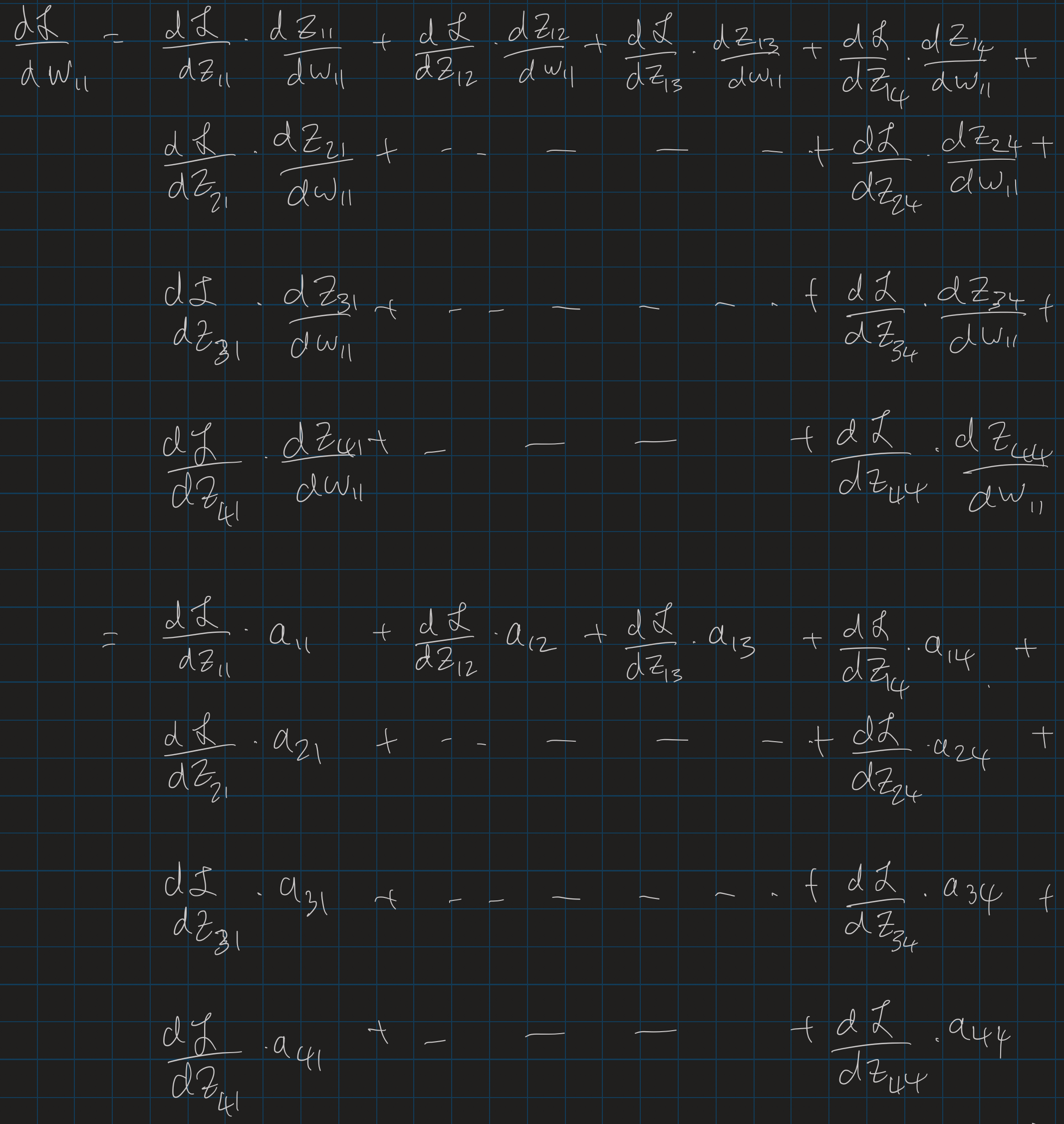
If we want the total \(\frac{\partial \mathcal{L}}{\partial W^{[2]}_{1, 1}}\) we just need to sum this across all paths, or all elements \(z^{[2]}_{k, l}\) of \(z^{[2]}\):
$$ \begin{align} \frac{\partial \mathcal{L}}{\partial W^{[2]}_{1, 1}} &= \sum_{k, l} \frac{\partial \mathcal{L}}{\partial z^{[2]}_{k, l}}\frac{\partial z^{[2]}_{k, l}}{\partial W^{[2]}_{1, 1}}\\[2em] &= \frac{\partial \mathcal{L}}{\partial z^{[2]}_{1, 1}}\frac{\partial z^{[2]}_{1, 1}}{\partial W^{[2]}_{1, 1}} + \frac{\partial \mathcal{L}}{\partial z^{[2]}_{12}}\frac{\partial z^{[2]}_{12}}{\partial W^{[2]}_{1, 1}} + \cdots + \frac{\partial \mathcal{L}}{\partial z^{[2]}_{44}}\frac{\partial z^{[2]}_{44}}{\partial W^{[2]}_{1, 1}} \end{align} $$
Generalizing from \(W^{[2]}_{1, 1}\) to any element, \(W^{[2]}_{i, j}\) of \(W^{[2]}\):
$$ \frac{\partial \mathcal{L}}{\partial W^{[2]}_{i, j}} = \sum_{k, l} \frac{\partial \mathcal{L}}{\partial z^{[2]}_{k, l}}\frac{\partial z^{[2]}_{k, l}}{\partial W^{[2]}_{i, j}} $$
We could of course work out by hand what this expression reduces to. But we’ve got a whole symbolic engine at our disposal - lets use it instead!
*If some element, \(z^{[2]}_{k, l}\), of \(z^{[2]}\) somehow didn’t contribute to the loss (say due to dropout or something else impeding the path to between \(z^{[2]}_{k, l}\) and the output) then the value of \(\frac{\partial \mathcal{L}}{\partial z^{[2]}_{k, l}}\) would be zero. We’re assuming all elements of \(\frac{\partial \mathcal{L}}{\partial z^{[2]}}\) are given to us correctly, so as long as all contributions of \(z^{[2]}_{k, l}\) to the loss are expressed in terms of \(\frac{\partial \mathcal{L}}{\partial z^{[2]}_{k, l}}\), the calculations will work out even if \(z^{[2]}_{k, l}\) has no impact on the loss.
Automatic Differentiation in SymPy 🔗
Earlier, I alluded to SymPy’s ability to do calculus. Let’s look at one of those abilities - differentiation - in more detail. Here’s a quick showcase: let’s create a symbolic expression for: \(x = 2y^2 + 3z\) and then differentiate with respect to \(y\):
x, y, z = symbols('x y z')
x = 2*y**2 + 3*z
x.diff(y)
\(\displaystyle 4 y\)
The answer, \(4y\), is of course what we expect.
In the computation of \(\frac{\partial \mathcal{L}}{\partial W^{[2]}_{i, j}}\) in the previous section, we needed \(\frac{\partial z^{[2]}_{k, l}}{\partial W^{[2]}_{i, j}}\). Our z2 matrix already contains the expressions for each element of \(z^{[2]}\). E.g. \(z^{[2]}_{1, 1}\) is:
z2[0][0]
\(\displaystyle b^{[2]} + {W^{[2]}}_{1,1} {a^{[1]}}_{1,1} + {W^{[2]}}_{1,2} {a^{[1]}}_{1,2} + {W^{[2]}}_{1,3} {a^{[1]}}_{1,3} + {W^{[2]}}_{2,1} {a^{[1]}}_{2,1} + {W^{[2]}}_{2,2} {a^{[1]}}_{2,2} + {W^{[2]}}_{2,3} {a^{[1]}}_{2,3} + {W^{[2]}}_{3,1} {a^{[1]}}_{3,1} + {W^{[2]}}_{3,2} {a^{[1]}}_{3,2} + {W^{[2]}}_{3,3} {a^{[1]}}_{3,3}\)
We can use the same diff() method shown in the example above to compute the derivatives with respect to the elements of \(W^{[2]}\). E.g., here’s \(\frac{\partial z^{[2]}_{1, 1}}{\partial W^{[2]}_{1, 1}}\)
z2[0][0].diff(W2[0][0])
\(\displaystyle {a^{[1]}}_{1,1}\)
We could now write some code to compute each element of \(\frac{\partial \mathcal{L}}{\partial W^{[2]}}\) by applying the chain rule with each element of \(\frac{\partial \mathcal{L}}{\partial z^{[2]}}\) and summing, as we worked out above. But we’re going to need similar logic in other cases, so let’s write a more general-purpose chain_rule() function we can re-use.
def chain_rule(dxs_and_xs: Iterable[Tuple[Expr, Expr]], t: Expr) -> Expr:
    """Say f is a function of variables x_1, x_2, ... x_n and each x_i is
    is a function of some other variable t. This function computes the
    general form of the chain rule:

    df/dt = df/dx_1 * dx_1/dt + df/dx_2 * dx_2/dt + ... + df/dx_n * dx_n/dt

    Params:
        dxs_and_xs: An iterable of tuples where the first element is an
                    expression for df/dx_i and the second element is an
                    expression for x_i. So this param would be structured
                    like:

                    [(df_dx1, x1), (df_dx2, x2), ..., (df_dxn, xn)]

        t:          Expression for variable t
    """
    return sum(dx * x.diff(t) for dx, x in dxs_and_xs)
Now, let’s use our symbolic engine and our chain_rule() function to work out \(\frac{\partial \mathcal{L}}{\partial W^{[2]}}\).
# Describe the loss function symbolically
y = symbols('y')
yhat = symbols(r'\hat{y}')
L = Function(r'\mathcal{L}')(y, yhat)

# Build dL/dz2
dz2 = ndarray_of_indexed_base(
    IndexedBase(r'z^{[2]}'), z2.shape, transform=lambda x: Derivative(L, x)
)

# Create a ufunc that can be broadcast across an ndarray and applies
# chain_rule() with dz2 and z2 across all elements.
dz2_chain_rule_ufunc = np.frompyfunc(
    lambda x: chain_rule(zip(dz2.reshape(-1), z2.reshape(-1)), x), 1, 1
)

# Calculate dW2 (look how nice this is!)
dW2 = dz2_chain_rule_ufunc(W2)

Markdown(matrix_to_markdown(dW2))
$$\begin{bmatrix} \frac{\partial}{\partial {z^{[2]}}_{1,1}} \mathcal{L}{\left(y,\hat{y} \right)} {a^{[1]}}_{1,1} + \frac{\partial}{\partial {z^{[2]}}_{1,2}} \mathcal{L}{\left(y,\hat{y} \right)} {a^{[1]}}_{1,2} + \frac{\partial}{\partial {z^{[2]}}_{1,3}} \mathcal{L}{\left(y,\hat{y} \right)} {a^{[1]}}_{1,3} + \frac{\partial}{\partial {z^{[2]}}_{1,4}} \mathcal{L}{\left(y,\hat{y} \right)} {a^{[1]}}_{1,4} + \frac{\partial}{\partial {z^{[2]}}_{2,1}} \mathcal{L}{\left(y,\hat{y} \right)} {a^{[1]}}_{2,1} + \frac{\partial}{\partial {z^{[2]}}_{2,2}} \mathcal{L}{\left(y,\hat{y} \right)} {a^{[1]}}_{2,2} + \frac{\partial}{\partial {z^{[2]}}_{2,3}} \mathcal{L}{\left(y,\hat{y} \right)} {a^{[1]}}_{2,3} + \frac{\partial}{\partial {z^{[2]}}_{2,4}} \mathcal{L}{\left(y,\hat{y} \right)} {a^{[1]}}_{2,4} + \frac{\partial}{\partial {z^{[2]}}_{3,1}} \mathcal{L}{\left(y,\hat{y} \right)} {a^{[1]}}_{3,1} + \frac{\partial}{\partial {z^{[2]}}_{3,2}} \mathcal{L}{\left(y,\hat{y} \right)} {a^{[1]}}_{3,2} + \frac{\partial}{\partial {z^{[2]}}_{3,3}} \mathcal{L}{\left(y,\hat{y} \right)} {a^{[1]}}_{3,3} + \frac{\partial}{\partial {z^{[2]}}_{3,4}} \mathcal{L}{\left(y,\hat{y} \right)} {a^{[1]}}_{3,4} + \frac{\partial}{\partial {z^{[2]}}_{4,1}} \mathcal{L}{\left(y,\hat{y} \right)} {a^{[1]}}_{4,1} + \frac{\partial}{\partial {z^{[2]}}_{4,2}} \mathcal{L}{\left(y,\hat{y} \right)} {a^{[1]}}_{4,2} + \frac{\partial}{\partial {z^{[2]}}_{4,3}} \mathcal{L}{\left(y,\hat{y} \right)} {a^{[1]}}_{4,3} + \frac{\partial}{\partial {z^{[2]}}_{4,4}} \mathcal{L}{\left(y,\hat{y} \right)} {a^{[1]}}_{4,4} & \frac{\partial}{\partial {z^{[2]}}_{1,1}} \mathcal{L}{\left(y,\hat{y} \right)} {a^{[1]}}_{1,2} + \frac{\partial}{\partial {z^{[2]}}_{1,2}} \mathcal{L}{\left(y,\hat{y} \right)} {a^{[1]}}_{1,3} + \frac{\partial}{\partial {z^{[2]}}_{1,3}} \mathcal{L}{\left(y,\hat{y} \right)} {a^{[1]}}_{1,4} + \frac{\partial}{\partial {z^{[2]}}_{1,4}} \mathcal{L}{\left(y,\hat{y} \right)} {a^{[1]}}_{1,5} + \frac{\partial}{\partial {z^{[2]}}_{2,1}} \mathcal{L}{\left(y,\hat{y} \right)} {a^{[1]}}_{2,2} + \frac{\partial}{\partial {z^{[2]}}_{2,2}} \mathcal{L}{\left(y,\hat{y} \right)} {a^{[1]}}_{2,3} + \frac{\partial}{\partial {z^{[2]}}_{2,3}} \mathcal{L}{\left(y,\hat{y} \right)} {a^{[1]}}_{2,4} + \frac{\partial}{\partial {z^{[2]}}_{2,4}} \mathcal{L}{\left(y,\hat{y} \right)} {a^{[1]}}_{2,5} + \frac{\partial}{\partial {z^{[2]}}_{3,1}} \mathcal{L}{\left(y,\hat{y} \right)} {a^{[1]}}_{3,2} + \frac{\partial}{\partial {z^{[2]}}_{3,2}} \mathcal{L}{\left(y,\hat{y} \right)} {a^{[1]}}_{3,3} + \frac{\partial}{\partial {z^{[2]}}_{3,3}} \mathcal{L}{\left(y,\hat{y} \right)} {a^{[1]}}_{3,4} + \frac{\partial}{\partial {z^{[2]}}_{3,4}} \mathcal{L}{\left(y,\hat{y} \right)} {a^{[1]}}_{3,5} + \frac{\partial}{\partial {z^{[2]}}_{4,1}} \mathcal{L}{\left(y,\hat{y} \right)} {a^{[1]}}_{4,2} + \frac{\partial}{\partial {z^{[2]}}_{4,2}} \mathcal{L}{\left(y,\hat{y} \right)} {a^{[1]}}_{4,3} + \frac{\partial}{\partial {z^{[2]}}_{4,3}} \mathcal{L}{\left(y,\hat{y} \right)} {a^{[1]}}_{4,4} + \frac{\partial}{\partial {z^{[2]}}_{4,4}} \mathcal{L}{\left(y,\hat{y} \right)} {a^{[1]}}_{4,5} & \frac{\partial}{\partial {z^{[2]}}_{1,1}} \mathcal{L}{\left(y,\hat{y} \right)} {a^{[1]}}_{1,3} + \frac{\partial}{\partial {z^{[2]}}_{1,2}} \mathcal{L}{\left(y,\hat{y} \right)} {a^{[1]}}_{1,4} + \frac{\partial}{\partial {z^{[2]}}_{1,3}} \mathcal{L}{\left(y,\hat{y} \right)} {a^{[1]}}_{1,5} + \frac{\partial}{\partial {z^{[2]}}_{1,4}} \mathcal{L}{\left(y,\hat{y} \right)} {a^{[1]}}_{1,6} + \frac{\partial}{\partial {z^{[2]}}_{2,1}} \mathcal{L}{\left(y,\hat{y} \right)} {a^{[1]}}_{2,3} + \frac{\partial}{\partial {z^{[2]}}_{2,2}} \mathcal{L}{\left(y,\hat{y} \right)} {a^{[1]}}_{2,4} + \frac{\partial}{\partial {z^{[2]}}_{2,3}} \mathcal{L}{\left(y,\hat{y} \right)} {a^{[1]}}_{2,5} + \frac{\partial}{\partial {z^{[2]}}_{2,4}} \mathcal{L}{\left(y,\hat{y} \right)} {a^{[1]}}_{2,6} + \frac{\partial}{\partial {z^{[2]}}_{3,1}} \mathcal{L}{\left(y,\hat{y} \right)} {a^{[1]}}_{3,3} + \frac{\partial}{\partial {z^{[2]}}_{3,2}} \mathcal{L}{\left(y,\hat{y} \right)} {a^{[1]}}_{3,4} + \frac{\partial}{\partial {z^{[2]}}_{3,3}} \mathcal{L}{\left(y,\hat{y} \right)} {a^{[1]}}_{3,5} + \frac{\partial}{\partial {z^{[2]}}_{3,4}} \mathcal{L}{\left(y,\hat{y} \right)} {a^{[1]}}_{3,6} + \frac{\partial}{\partial {z^{[2]}}_{4,1}} \mathcal{L}{\left(y,\hat{y} \right)} {a^{[1]}}_{4,3} + \frac{\partial}{\partial {z^{[2]}}_{4,2}} \mathcal{L}{\left(y,\hat{y} \right)} {a^{[1]}}_{4,4} + \frac{\partial}{\partial {z^{[2]}}_{4,3}} \mathcal{L}{\left(y,\hat{y} \right)} {a^{[1]}}_{4,5} + \frac{\partial}{\partial {z^{[2]}}_{4,4}} \mathcal{L}{\left(y,\hat{y} \right)} {a^{[1]}}_{4,6}\\ \frac{\partial}{\partial {z^{[2]}}_{1,1}} \mathcal{L}{\left(y,\hat{y} \right)} {a^{[1]}}_{2,1} + \frac{\partial}{\partial {z^{[2]}}_{1,2}} \mathcal{L}{\left(y,\hat{y} \right)} {a^{[1]}}_{2,2} + \frac{\partial}{\partial {z^{[2]}}_{1,3}} \mathcal{L}{\left(y,\hat{y} \right)} {a^{[1]}}_{2,3} + \frac{\partial}{\partial {z^{[2]}}_{1,4}} \mathcal{L}{\left(y,\hat{y} \right)} {a^{[1]}}_{2,4} + \frac{\partial}{\partial {z^{[2]}}_{2,1}} \mathcal{L}{\left(y,\hat{y} \right)} {a^{[1]}}_{3,1} + \frac{\partial}{\partial {z^{[2]}}_{2,2}} \mathcal{L}{\left(y,\hat{y} \right)} {a^{[1]}}_{3,2} + \frac{\partial}{\partial {z^{[2]}}_{2,3}} \mathcal{L}{\left(y,\hat{y} \right)} {a^{[1]}}_{3,3} + \frac{\partial}{\partial {z^{[2]}}_{2,4}} \mathcal{L}{\left(y,\hat{y} \right)} {a^{[1]}}_{3,4} + \frac{\partial}{\partial {z^{[2]}}_{3,1}} \mathcal{L}{\left(y,\hat{y} \right)} {a^{[1]}}_{4,1} + \frac{\partial}{\partial {z^{[2]}}_{3,2}} \mathcal{L}{\left(y,\hat{y} \right)} {a^{[1]}}_{4,2} + \frac{\partial}{\partial {z^{[2]}}_{3,3}} \mathcal{L}{\left(y,\hat{y} \right)} {a^{[1]}}_{4,3} + \frac{\partial}{\partial {z^{[2]}}_{3,4}} \mathcal{L}{\left(y,\hat{y} \right)} {a^{[1]}}_{4,4} + \frac{\partial}{\partial {z^{[2]}}_{4,1}} \mathcal{L}{\left(y,\hat{y} \right)} {a^{[1]}}_{5,1} + \frac{\partial}{\partial {z^{[2]}}_{4,2}} \mathcal{L}{\left(y,\hat{y} \right)} {a^{[1]}}_{5,2} + \frac{\partial}{\partial {z^{[2]}}_{4,3}} \mathcal{L}{\left(y,\hat{y} \right)} {a^{[1]}}_{5,3} + \frac{\partial}{\partial {z^{[2]}}_{4,4}} \mathcal{L}{\left(y,\hat{y} \right)} {a^{[1]}}_{5,4} & \frac{\partial}{\partial {z^{[2]}}_{1,1}} \mathcal{L}{\left(y,\hat{y} \right)} {a^{[1]}}_{2,2} + \frac{\partial}{\partial {z^{[2]}}_{1,2}} \mathcal{L}{\left(y,\hat{y} \right)} {a^{[1]}}_{2,3} + \frac{\partial}{\partial {z^{[2]}}_{1,3}} \mathcal{L}{\left(y,\hat{y} \right)} {a^{[1]}}_{2,4} + \frac{\partial}{\partial {z^{[2]}}_{1,4}} \mathcal{L}{\left(y,\hat{y} \right)} {a^{[1]}}_{2,5} + \frac{\partial}{\partial {z^{[2]}}_{2,1}} \mathcal{L}{\left(y,\hat{y} \right)} {a^{[1]}}_{3,2} + \frac{\partial}{\partial {z^{[2]}}_{2,2}} \mathcal{L}{\left(y,\hat{y} \right)} {a^{[1]}}_{3,3} + \frac{\partial}{\partial {z^{[2]}}_{2,3}} \mathcal{L}{\left(y,\hat{y} \right)} {a^{[1]}}_{3,4} + \frac{\partial}{\partial {z^{[2]}}_{2,4}} \mathcal{L}{\left(y,\hat{y} \right)} {a^{[1]}}_{3,5} + \frac{\partial}{\partial {z^{[2]}}_{3,1}} \mathcal{L}{\left(y,\hat{y} \right)} {a^{[1]}}_{4,2} + \frac{\partial}{\partial {z^{[2]}}_{3,2}} \mathcal{L}{\left(y,\hat{y} \right)} {a^{[1]}}_{4,3} + \frac{\partial}{\partial {z^{[2]}}_{3,3}} \mathcal{L}{\left(y,\hat{y} \right)} {a^{[1]}}_{4,4} + \frac{\partial}{\partial {z^{[2]}}_{3,4}} \mathcal{L}{\left(y,\hat{y} \right)} {a^{[1]}}_{4,5} + \frac{\partial}{\partial {z^{[2]}}_{4,1}} \mathcal{L}{\left(y,\hat{y} \right)} {a^{[1]}}_{5,2} + \frac{\partial}{\partial {z^{[2]}}_{4,2}} \mathcal{L}{\left(y,\hat{y} \right)} {a^{[1]}}_{5,3} + \frac{\partial}{\partial {z^{[2]}}_{4,3}} \mathcal{L}{\left(y,\hat{y} \right)} {a^{[1]}}_{5,4} + \frac{\partial}{\partial {z^{[2]}}_{4,4}} \mathcal{L}{\left(y,\hat{y} \right)} {a^{[1]}}_{5,5} & \frac{\partial}{\partial {z^{[2]}}_{1,1}} \mathcal{L}{\left(y,\hat{y} \right)} {a^{[1]}}_{2,3} + \frac{\partial}{\partial {z^{[2]}}_{1,2}} \mathcal{L}{\left(y,\hat{y} \right)} {a^{[1]}}_{2,4} + \frac{\partial}{\partial {z^{[2]}}_{1,3}} \mathcal{L}{\left(y,\hat{y} \right)} {a^{[1]}}_{2,5} + \frac{\partial}{\partial {z^{[2]}}_{1,4}} \mathcal{L}{\left(y,\hat{y} \right)} {a^{[1]}}_{2,6} + \frac{\partial}{\partial {z^{[2]}}_{2,1}} \mathcal{L}{\left(y,\hat{y} \right)} {a^{[1]}}_{3,3} + \frac{\partial}{\partial {z^{[2]}}_{2,2}} \mathcal{L}{\left(y,\hat{y} \right)} {a^{[1]}}_{3,4} + \frac{\partial}{\partial {z^{[2]}}_{2,3}} \mathcal{L}{\left(y,\hat{y} \right)} {a^{[1]}}_{3,5} + \frac{\partial}{\partial {z^{[2]}}_{2,4}} \mathcal{L}{\left(y,\hat{y} \right)} {a^{[1]}}_{3,6} + \frac{\partial}{\partial {z^{[2]}}_{3,1}} \mathcal{L}{\left(y,\hat{y} \right)} {a^{[1]}}_{4,3} + \frac{\partial}{\partial {z^{[2]}}_{3,2}} \mathcal{L}{\left(y,\hat{y} \right)} {a^{[1]}}_{4,4} + \frac{\partial}{\partial {z^{[2]}}_{3,3}} \mathcal{L}{\left(y,\hat{y} \right)} {a^{[1]}}_{4,5} + \frac{\partial}{\partial {z^{[2]}}_{3,4}} \mathcal{L}{\left(y,\hat{y} \right)} {a^{[1]}}_{4,6} + \frac{\partial}{\partial {z^{[2]}}_{4,1}} \mathcal{L}{\left(y,\hat{y} \right)} {a^{[1]}}_{5,3} + \frac{\partial}{\partial {z^{[2]}}_{4,2}} \mathcal{L}{\left(y,\hat{y} \right)} {a^{[1]}}_{5,4} + \frac{\partial}{\partial {z^{[2]}}_{4,3}} \mathcal{L}{\left(y,\hat{y} \right)} {a^{[1]}}_{5,5} + \frac{\partial}{\partial {z^{[2]}}_{4,4}} \mathcal{L}{\left(y,\hat{y} \right)} {a^{[1]}}_{5,6}\\ \frac{\partial}{\partial {z^{[2]}}_{1,1}} \mathcal{L}{\left(y,\hat{y} \right)} {a^{[1]}}_{3,1} + \frac{\partial}{\partial {z^{[2]}}_{1,2}} \mathcal{L}{\left(y,\hat{y} \right)} {a^{[1]}}_{3,2} + \frac{\partial}{\partial {z^{[2]}}_{1,3}} \mathcal{L}{\left(y,\hat{y} \right)} {a^{[1]}}_{3,3} + \frac{\partial}{\partial {z^{[2]}}_{1,4}} \mathcal{L}{\left(y,\hat{y} \right)} {a^{[1]}}_{3,4} + \frac{\partial}{\partial {z^{[2]}}_{2,1}} \mathcal{L}{\left(y,\hat{y} \right)} {a^{[1]}}_{4,1} + \frac{\partial}{\partial {z^{[2]}}_{2,2}} \mathcal{L}{\left(y,\hat{y} \right)} {a^{[1]}}_{4,2} + \frac{\partial}{\partial {z^{[2]}}_{2,3}} \mathcal{L}{\left(y,\hat{y} \right)} {a^{[1]}}_{4,3} + \frac{\partial}{\partial {z^{[2]}}_{2,4}} \mathcal{L}{\left(y,\hat{y} \right)} {a^{[1]}}_{4,4} + \frac{\partial}{\partial {z^{[2]}}_{3,1}} \mathcal{L}{\left(y,\hat{y} \right)} {a^{[1]}}_{5,1} + \frac{\partial}{\partial {z^{[2]}}_{3,2}} \mathcal{L}{\left(y,\hat{y} \right)} {a^{[1]}}_{5,2} + \frac{\partial}{\partial {z^{[2]}}_{3,3}} \mathcal{L}{\left(y,\hat{y} \right)} {a^{[1]}}_{5,3} + \frac{\partial}{\partial {z^{[2]}}_{3,4}} \mathcal{L}{\left(y,\hat{y} \right)} {a^{[1]}}_{5,4} + \frac{\partial}{\partial {z^{[2]}}_{4,1}} \mathcal{L}{\left(y,\hat{y} \right)} {a^{[1]}}_{6,1} + \frac{\partial}{\partial {z^{[2]}}_{4,2}} \mathcal{L}{\left(y,\hat{y} \right)} {a^{[1]}}_{6,2} + \frac{\partial}{\partial {z^{[2]}}_{4,3}} \mathcal{L}{\left(y,\hat{y} \right)} {a^{[1]}}_{6,3} + \frac{\partial}{\partial {z^{[2]}}_{4,4}} \mathcal{L}{\left(y,\hat{y} \right)} {a^{[1]}}_{6,4} & \frac{\partial}{\partial {z^{[2]}}_{1,1}} \mathcal{L}{\left(y,\hat{y} \right)} {a^{[1]}}_{3,2} + \frac{\partial}{\partial {z^{[2]}}_{1,2}} \mathcal{L}{\left(y,\hat{y} \right)} {a^{[1]}}_{3,3} + \frac{\partial}{\partial {z^{[2]}}_{1,3}} \mathcal{L}{\left(y,\hat{y} \right)} {a^{[1]}}_{3,4} + \frac{\partial}{\partial {z^{[2]}}_{1,4}} \mathcal{L}{\left(y,\hat{y} \right)} {a^{[1]}}_{3,5} + \frac{\partial}{\partial {z^{[2]}}_{2,1}} \mathcal{L}{\left(y,\hat{y} \right)} {a^{[1]}}_{4,2} + \frac{\partial}{\partial {z^{[2]}}_{2,2}} \mathcal{L}{\left(y,\hat{y} \right)} {a^{[1]}}_{4,3} + \frac{\partial}{\partial {z^{[2]}}_{2,3}} \mathcal{L}{\left(y,\hat{y} \right)} {a^{[1]}}_{4,4} + \frac{\partial}{\partial {z^{[2]}}_{2,4}} \mathcal{L}{\left(y,\hat{y} \right)} {a^{[1]}}_{4,5} + \frac{\partial}{\partial {z^{[2]}}_{3,1}} \mathcal{L}{\left(y,\hat{y} \right)} {a^{[1]}}_{5,2} + \frac{\partial}{\partial {z^{[2]}}_{3,2}} \mathcal{L}{\left(y,\hat{y} \right)} {a^{[1]}}_{5,3} + \frac{\partial}{\partial {z^{[2]}}_{3,3}} \mathcal{L}{\left(y,\hat{y} \right)} {a^{[1]}}_{5,4} + \frac{\partial}{\partial {z^{[2]}}_{3,4}} \mathcal{L}{\left(y,\hat{y} \right)} {a^{[1]}}_{5,5} + \frac{\partial}{\partial {z^{[2]}}_{4,1}} \mathcal{L}{\left(y,\hat{y} \right)} {a^{[1]}}_{6,2} + \frac{\partial}{\partial {z^{[2]}}_{4,2}} \mathcal{L}{\left(y,\hat{y} \right)} {a^{[1]}}_{6,3} + \frac{\partial}{\partial {z^{[2]}}_{4,3}} \mathcal{L}{\left(y,\hat{y} \right)} {a^{[1]}}_{6,4} + \frac{\partial}{\partial {z^{[2]}}_{4,4}} \mathcal{L}{\left(y,\hat{y} \right)} {a^{[1]}}_{6,5} & \frac{\partial}{\partial {z^{[2]}}_{1,1}} \mathcal{L}{\left(y,\hat{y} \right)} {a^{[1]}}_{3,3} + \frac{\partial}{\partial {z^{[2]}}_{1,2}} \mathcal{L}{\left(y,\hat{y} \right)} {a^{[1]}}_{3,4} + \frac{\partial}{\partial {z^{[2]}}_{1,3}} \mathcal{L}{\left(y,\hat{y} \right)} {a^{[1]}}_{3,5} + \frac{\partial}{\partial {z^{[2]}}_{1,4}} \mathcal{L}{\left(y,\hat{y} \right)} {a^{[1]}}_{3,6} + \frac{\partial}{\partial {z^{[2]}}_{2,1}} \mathcal{L}{\left(y,\hat{y} \right)} {a^{[1]}}_{4,3} + \frac{\partial}{\partial {z^{[2]}}_{2,2}} \mathcal{L}{\left(y,\hat{y} \right)} {a^{[1]}}_{4,4} + \frac{\partial}{\partial {z^{[2]}}_{2,3}} \mathcal{L}{\left(y,\hat{y} \right)} {a^{[1]}}_{4,5} + \frac{\partial}{\partial {z^{[2]}}_{2,4}} \mathcal{L}{\left(y,\hat{y} \right)} {a^{[1]}}_{4,6} + \frac{\partial}{\partial {z^{[2]}}_{3,1}} \mathcal{L}{\left(y,\hat{y} \right)} {a^{[1]}}_{5,3} + \frac{\partial}{\partial {z^{[2]}}_{3,2}} \mathcal{L}{\left(y,\hat{y} \right)} {a^{[1]}}_{5,4} + \frac{\partial}{\partial {z^{[2]}}_{3,3}} \mathcal{L}{\left(y,\hat{y} \right)} {a^{[1]}}_{5,5} + \frac{\partial}{\partial {z^{[2]}}_{3,4}} \mathcal{L}{\left(y,\hat{y} \right)} {a^{[1]}}_{5,6} + \frac{\partial}{\partial {z^{[2]}}_{4,1}} \mathcal{L}{\left(y,\hat{y} \right)} {a^{[1]}}_{6,3} + \frac{\partial}{\partial {z^{[2]}}_{4,2}} \mathcal{L}{\left(y,\hat{y} \right)} {a^{[1]}}_{6,4} + \frac{\partial}{\partial {z^{[2]}}_{4,3}} \mathcal{L}{\left(y,\hat{y} \right)} {a^{[1]}}_{6,5} + \frac{\partial}{\partial {z^{[2]}}_{4,4}} \mathcal{L}{\left(y,\hat{y} \right)} {a^{[1]}}_{6,6}\end{bmatrix} $$
OK, we got a matrix, and each element of this is an expression. Before trying to dig into it, let’s just visualize it. Each expression looks like a sum of products and so like before, we can build a highlight map from it, and use this to animate a diagram. But we do need to make one tiny change to build_highlights_map(), to make it deal with the derivatives of indexed objects.
def build_highlights_map(expr: Expr) -> Dict[str, List[Tuple]]:
    # The expression needs to be either a sum of products or a single product
    assert expr.func == Add or expr.func == Mul

    # If it's an Add, assert all args are Muls
    if expr.func == Add:
        assert all(arg.func == Mul for arg in expr.args)

    # We want the list of multiplications. This is either a list consisting
    # of just the expression itself if it's a Mul or its arguments if it's
    # an Add.
    muls = [expr] if expr.func == Mul else expr.args

    results = {}
    for expr in muls:
        # Assert all the args are Indexed or derivatives w.r.t. an Indexed
        assert all(
            arg.func == Indexed
            or (arg.func == Derivative and arg.args[1][0].func == Indexed)
            for arg in expr.args
        )

        indexeds = [arg if arg.func == Indexed else arg.args[1][0] for arg in expr.args]

        for indexed in indexeds:
            if indexed.base.name not in results:
                results[indexed.base.name] = []
            results[indexed.base.name].append(indexed.indices)
    return results
We can now use this version of build_highlights_map() in drawing code to visualize the operations used to compute \(\frac{\partial \mathcal{L}}{\partial W^{[2]}}\). The result is the video below.
This looks a whole lot like a convolution of \(a^{[1]}\) with \(\frac{\partial \mathcal{L}}{\partial z^{[2]}}\). We can confirm this with the equations:
display(dW2[0][0])
\(\displaystyle \frac{\partial}{\partial {z^{[2]}}_{1,1}} \mathcal{L}{\left(y,\hat{y} \right)} {a^{[1]}}_{1,1} + \frac{\partial}{\partial {z^{[2]}}_{1,2}} \mathcal{L}{\left(y,\hat{y} \right)} {a^{[1]}}_{1,2} + \frac{\partial}{\partial {z^{[2]}}_{1,3}} \mathcal{L}{\left(y,\hat{y} \right)} {a^{[1]}}_{1,3} + \frac{\partial}{\partial {z^{[2]}}_{1,4}} \mathcal{L}{\left(y,\hat{y} \right)} {a^{[1]}}_{1,4} + \frac{\partial}{\partial {z^{[2]}}_{2,1}} \mathcal{L}{\left(y,\hat{y} \right)} {a^{[1]}}_{2,1} + \frac{\partial}{\partial {z^{[2]}}_{2,2}} \mathcal{L}{\left(y,\hat{y} \right)} {a^{[1]}}_{2,2} + \frac{\partial}{\partial {z^{[2]}}_{2,3}} \mathcal{L}{\left(y,\hat{y} \right)} {a^{[1]}}_{2,3} + \frac{\partial}{\partial {z^{[2]}}_{2,4}} \mathcal{L}{\left(y,\hat{y} \right)} {a^{[1]}}_{2,4} + \frac{\partial}{\partial {z^{[2]}}_{3,1}} \mathcal{L}{\left(y,\hat{y} \right)} {a^{[1]}}_{3,1} + \frac{\partial}{\partial {z^{[2]}}_{3,2}} \mathcal{L}{\left(y,\hat{y} \right)} {a^{[1]}}_{3,2} + \frac{\partial}{\partial {z^{[2]}}_{3,3}} \mathcal{L}{\left(y,\hat{y} \right)} {a^{[1]}}_{3,3} + \frac{\partial}{\partial {z^{[2]}}_{3,4}} \mathcal{L}{\left(y,\hat{y} \right)} {a^{[1]}}_{3,4} + \frac{\partial}{\partial {z^{[2]}}_{4,1}} \mathcal{L}{\left(y,\hat{y} \right)} {a^{[1]}}_{4,1} + \frac{\partial}{\partial {z^{[2]}}_{4,2}} \mathcal{L}{\left(y,\hat{y} \right)} {a^{[1]}}_{4,2} + \frac{\partial}{\partial {z^{[2]}}_{4,3}} \mathcal{L}{\left(y,\hat{y} \right)} {a^{[1]}}_{4,3} + \frac{\partial}{\partial {z^{[2]}}_{4,4}} \mathcal{L}{\left(y,\hat{y} \right)} {a^{[1]}}_{4,4}\)
display(dW2[1][0])
\(\displaystyle \frac{\partial}{\partial {z^{[2]}}_{1,1}} \mathcal{L}{\left(y,\hat{y} \right)} {a^{[1]}}_{2,1} + \frac{\partial}{\partial {z^{[2]}}_{1,2}} \mathcal{L}{\left(y,\hat{y} \right)} {a^{[1]}}_{2,2} + \frac{\partial}{\partial {z^{[2]}}_{1,3}} \mathcal{L}{\left(y,\hat{y} \right)} {a^{[1]}}_{2,3} + \frac{\partial}{\partial {z^{[2]}}_{1,4}} \mathcal{L}{\left(y,\hat{y} \right)} {a^{[1]}}_{2,4} + \frac{\partial}{\partial {z^{[2]}}_{2,1}} \mathcal{L}{\left(y,\hat{y} \right)} {a^{[1]}}_{3,1} + \frac{\partial}{\partial {z^{[2]}}_{2,2}} \mathcal{L}{\left(y,\hat{y} \right)} {a^{[1]}}_{3,2} + \frac{\partial}{\partial {z^{[2]}}_{2,3}} \mathcal{L}{\left(y,\hat{y} \right)} {a^{[1]}}_{3,3} + \frac{\partial}{\partial {z^{[2]}}_{2,4}} \mathcal{L}{\left(y,\hat{y} \right)} {a^{[1]}}_{3,4} + \frac{\partial}{\partial {z^{[2]}}_{3,1}} \mathcal{L}{\left(y,\hat{y} \right)} {a^{[1]}}_{4,1} + \frac{\partial}{\partial {z^{[2]}}_{3,2}} \mathcal{L}{\left(y,\hat{y} \right)} {a^{[1]}}_{4,2} + \frac{\partial}{\partial {z^{[2]}}_{3,3}} \mathcal{L}{\left(y,\hat{y} \right)} {a^{[1]}}_{4,3} + \frac{\partial}{\partial {z^{[2]}}_{3,4}} \mathcal{L}{\left(y,\hat{y} \right)} {a^{[1]}}_{4,4} + \frac{\partial}{\partial {z^{[2]}}_{4,1}} \mathcal{L}{\left(y,\hat{y} \right)} {a^{[1]}}_{5,1} + \frac{\partial}{\partial {z^{[2]}}_{4,2}} \mathcal{L}{\left(y,\hat{y} \right)} {a^{[1]}}_{5,2} + \frac{\partial}{\partial {z^{[2]}}_{4,3}} \mathcal{L}{\left(y,\hat{y} \right)} {a^{[1]}}_{5,3} + \frac{\partial}{\partial {z^{[2]}}_{4,4}} \mathcal{L}{\left(y,\hat{y} \right)} {a^{[1]}}_{5,4}\)
Notice how in dw2[0][0] (which is \(\frac{\partial \mathcal{L}}{\partial W^{[2]}_{11}}\)) each element of \(\frac{\partial \mathcal{L}}{\partial z^{[2]}}\) is multiplied by the corresponding element of \(a^{[1]}\) and in dw2[1][0] (\(\frac{\partial \mathcal{L}}{\partial w^{[2]}_{21}}\)) all the indices of \(a^{[1]}\) are shifted down by one, as you’d expect.
But this is all so much easier to see in the visualization. Again, the visualization was generated from the expressions in dW2, not programmed based on some advanced knowledge of how it should look. In this way, it’s actually more of a simulation than a visualization.
Based on what we see in the visualization and our inspection of the equations, it seems:
$$ \frac{\partial \mathcal{L}}{\partial W^{[2]}} = a^{[1]} * \frac{\partial \mathcal{L}}{\partial z^{[2]}} $$
We can further convince ourselves by testing in code:
test_eq(convolve(a1, dz2, 0, 1), dW2)
Deriving \(\frac{\partial \mathcal{L}}{\partial a^{[1]}}\) 🔗
Next, let’s work out \(\frac{\partial \mathcal{L}}{\partial a^{[1]}}\), the gradient of the loss function with respect to the previous layer’s activations. Again, a computation graph helps visualize how the elements of \(a^{[1]}\) impact the loss:

It turns out we don’t have to think too hard about this. We can still apply the chain rule, as we did in the previous section. For each element \(a^{[1]}_{i, j}\) of \(a^{[1]}\):
$$ \frac{\partial \mathcal{L}}{\partial a^{[1]}_{i, j}} = \sum_{k, l} \frac{\partial \mathcal{L}}{\partial z^{[2]}_{k, l}}\frac{\partial z^{[2]}_{k, l}}{\partial a^{[1]}_{i, j}} $$
We’re summing across all possible paths from a given \(a^{[1]}_{i, j}\) through all the \(z^{[2]}_{k, l}\) terms to the loss. Because we actually have the expressions for each element of \(z^{[2]}\) in terms of the elements of \(W^{[2]}\) and \(a^{[1]}\), when some \(a^{[1]}_{i, j}\) does not contribute to some \(z^{[2]}_{k, l}\), the \(\frac{\partial z^{[2]}_{k, l}}{\partial a^{[1]}_{i, j}}\) term is zero. For example:
# a1[5][5] doesn't contribute to z2[0][0]
z2[0][0].diff(a1[5][5])
\(\displaystyle 0\)
So we can now compute all the elements of \(\frac{\partial \mathcal{L}}{\partial a^{[1]}}\) via the chain rule. And of course, we don’t have to do it by hand - the same chain rule helper function does the job.
da1 = dz2_chain_rule_ufunc(a1)

Markdown(matrix_to_markdown(da1))
$$\begin{bmatrix} \frac{\partial}{\partial {z^{[2]}}_{1,1}} \mathcal{L}{\left(y,\hat{y} \right)} {W^{[2]}}_{1,1} & \frac{\partial}{\partial {z^{[2]}}_{1,1}} \mathcal{L}{\left(y,\hat{y} \right)} {W^{[2]}}_{1,2} + \frac{\partial}{\partial {z^{[2]}}_{1,2}} \mathcal{L}{\left(y,\hat{y} \right)} {W^{[2]}}_{1,1} & \frac{\partial}{\partial {z^{[2]}}_{1,1}} \mathcal{L}{\left(y,\hat{y} \right)} {W^{[2]}}_{1,3} + \frac{\partial}{\partial {z^{[2]}}_{1,2}} \mathcal{L}{\left(y,\hat{y} \right)} {W^{[2]}}_{1,2} + \frac{\partial}{\partial {z^{[2]}}_{1,3}} \mathcal{L}{\left(y,\hat{y} \right)} {W^{[2]}}_{1,1} & \frac{\partial}{\partial {z^{[2]}}_{1,2}} \mathcal{L}{\left(y,\hat{y} \right)} {W^{[2]}}_{1,3} + \frac{\partial}{\partial {z^{[2]}}_{1,3}} \mathcal{L}{\left(y,\hat{y} \right)} {W^{[2]}}_{1,2} + \frac{\partial}{\partial {z^{[2]}}_{1,4}} \mathcal{L}{\left(y,\hat{y} \right)} {W^{[2]}}_{1,1} & \frac{\partial}{\partial {z^{[2]}}_{1,3}} \mathcal{L}{\left(y,\hat{y} \right)} {W^{[2]}}_{1,3} + \frac{\partial}{\partial {z^{[2]}}_{1,4}} \mathcal{L}{\left(y,\hat{y} \right)} {W^{[2]}}_{1,2} & \frac{\partial}{\partial {z^{[2]}}_{1,4}} \mathcal{L}{\left(y,\hat{y} \right)} {W^{[2]}}_{1,3}\\ \frac{\partial}{\partial {z^{[2]}}_{1,1}} \mathcal{L}{\left(y,\hat{y} \right)} {W^{[2]}}_{2,1} + \frac{\partial}{\partial {z^{[2]}}_{2,1}} \mathcal{L}{\left(y,\hat{y} \right)} {W^{[2]}}_{1,1} & \frac{\partial}{\partial {z^{[2]}}_{1,1}} \mathcal{L}{\left(y,\hat{y} \right)} {W^{[2]}}_{2,2} + \frac{\partial}{\partial {z^{[2]}}_{1,2}} \mathcal{L}{\left(y,\hat{y} \right)} {W^{[2]}}_{2,1} + \frac{\partial}{\partial {z^{[2]}}_{2,1}} \mathcal{L}{\left(y,\hat{y} \right)} {W^{[2]}}_{1,2} + \frac{\partial}{\partial {z^{[2]}}_{2,2}} \mathcal{L}{\left(y,\hat{y} \right)} {W^{[2]}}_{1,1} & \frac{\partial}{\partial {z^{[2]}}_{1,1}} \mathcal{L}{\left(y,\hat{y} \right)} {W^{[2]}}_{2,3} + \frac{\partial}{\partial {z^{[2]}}_{1,2}} \mathcal{L}{\left(y,\hat{y} \right)} {W^{[2]}}_{2,2} + \frac{\partial}{\partial {z^{[2]}}_{1,3}} \mathcal{L}{\left(y,\hat{y} \right)} {W^{[2]}}_{2,1} + \frac{\partial}{\partial {z^{[2]}}_{2,1}} \mathcal{L}{\left(y,\hat{y} \right)} {W^{[2]}}_{1,3} + \frac{\partial}{\partial {z^{[2]}}_{2,2}} \mathcal{L}{\left(y,\hat{y} \right)} {W^{[2]}}_{1,2} + \frac{\partial}{\partial {z^{[2]}}_{2,3}} \mathcal{L}{\left(y,\hat{y} \right)} {W^{[2]}}_{1,1} & \frac{\partial}{\partial {z^{[2]}}_{1,2}} \mathcal{L}{\left(y,\hat{y} \right)} {W^{[2]}}_{2,3} + \frac{\partial}{\partial {z^{[2]}}_{1,3}} \mathcal{L}{\left(y,\hat{y} \right)} {W^{[2]}}_{2,2} + \frac{\partial}{\partial {z^{[2]}}_{1,4}} \mathcal{L}{\left(y,\hat{y} \right)} {W^{[2]}}_{2,1} + \frac{\partial}{\partial {z^{[2]}}_{2,2}} \mathcal{L}{\left(y,\hat{y} \right)} {W^{[2]}}_{1,3} + \frac{\partial}{\partial {z^{[2]}}_{2,3}} \mathcal{L}{\left(y,\hat{y} \right)} {W^{[2]}}_{1,2} + \frac{\partial}{\partial {z^{[2]}}_{2,4}} \mathcal{L}{\left(y,\hat{y} \right)} {W^{[2]}}_{1,1} & \frac{\partial}{\partial {z^{[2]}}_{1,3}} \mathcal{L}{\left(y,\hat{y} \right)} {W^{[2]}}_{2,3} + \frac{\partial}{\partial {z^{[2]}}_{1,4}} \mathcal{L}{\left(y,\hat{y} \right)} {W^{[2]}}_{2,2} + \frac{\partial}{\partial {z^{[2]}}_{2,3}} \mathcal{L}{\left(y,\hat{y} \right)} {W^{[2]}}_{1,3} + \frac{\partial}{\partial {z^{[2]}}_{2,4}} \mathcal{L}{\left(y,\hat{y} \right)} {W^{[2]}}_{1,2} & \frac{\partial}{\partial {z^{[2]}}_{1,4}} \mathcal{L}{\left(y,\hat{y} \right)} {W^{[2]}}_{2,3} + \frac{\partial}{\partial {z^{[2]}}_{2,4}} \mathcal{L}{\left(y,\hat{y} \right)} {W^{[2]}}_{1,3}\\ \frac{\partial}{\partial {z^{[2]}}_{1,1}} \mathcal{L}{\left(y,\hat{y} \right)} {W^{[2]}}_{3,1} + \frac{\partial}{\partial {z^{[2]}}_{2,1}} \mathcal{L}{\left(y,\hat{y} \right)} {W^{[2]}}_{2,1} + \frac{\partial}{\partial {z^{[2]}}_{3,1}} \mathcal{L}{\left(y,\hat{y} \right)} {W^{[2]}}_{1,1} & \frac{\partial}{\partial {z^{[2]}}_{1,1}} \mathcal{L}{\left(y,\hat{y} \right)} {W^{[2]}}_{3,2} + \frac{\partial}{\partial {z^{[2]}}_{1,2}} \mathcal{L}{\left(y,\hat{y} \right)} {W^{[2]}}_{3,1} + \frac{\partial}{\partial {z^{[2]}}_{2,1}} \mathcal{L}{\left(y,\hat{y} \right)} {W^{[2]}}_{2,2} + \frac{\partial}{\partial {z^{[2]}}_{2,2}} \mathcal{L}{\left(y,\hat{y} \right)} {W^{[2]}}_{2,1} + \frac{\partial}{\partial {z^{[2]}}_{3,1}} \mathcal{L}{\left(y,\hat{y} \right)} {W^{[2]}}_{1,2} + \frac{\partial}{\partial {z^{[2]}}_{3,2}} \mathcal{L}{\left(y,\hat{y} \right)} {W^{[2]}}_{1,1} & \frac{\partial}{\partial {z^{[2]}}_{1,1}} \mathcal{L}{\left(y,\hat{y} \right)} {W^{[2]}}_{3,3} + \frac{\partial}{\partial {z^{[2]}}_{1,2}} \mathcal{L}{\left(y,\hat{y} \right)} {W^{[2]}}_{3,2} + \frac{\partial}{\partial {z^{[2]}}_{1,3}} \mathcal{L}{\left(y,\hat{y} \right)} {W^{[2]}}_{3,1} + \frac{\partial}{\partial {z^{[2]}}_{2,1}} \mathcal{L}{\left(y,\hat{y} \right)} {W^{[2]}}_{2,3} + \frac{\partial}{\partial {z^{[2]}}_{2,2}} \mathcal{L}{\left(y,\hat{y} \right)} {W^{[2]}}_{2,2} + \frac{\partial}{\partial {z^{[2]}}_{2,3}} \mathcal{L}{\left(y,\hat{y} \right)} {W^{[2]}}_{2,1} + \frac{\partial}{\partial {z^{[2]}}_{3,1}} \mathcal{L}{\left(y,\hat{y} \right)} {W^{[2]}}_{1,3} + \frac{\partial}{\partial {z^{[2]}}_{3,2}} \mathcal{L}{\left(y,\hat{y} \right)} {W^{[2]}}_{1,2} + \frac{\partial}{\partial {z^{[2]}}_{3,3}} \mathcal{L}{\left(y,\hat{y} \right)} {W^{[2]}}_{1,1} & \frac{\partial}{\partial {z^{[2]}}_{1,2}} \mathcal{L}{\left(y,\hat{y} \right)} {W^{[2]}}_{3,3} + \frac{\partial}{\partial {z^{[2]}}_{1,3}} \mathcal{L}{\left(y,\hat{y} \right)} {W^{[2]}}_{3,2} + \frac{\partial}{\partial {z^{[2]}}_{1,4}} \mathcal{L}{\left(y,\hat{y} \right)} {W^{[2]}}_{3,1} + \frac{\partial}{\partial {z^{[2]}}_{2,2}} \mathcal{L}{\left(y,\hat{y} \right)} {W^{[2]}}_{2,3} + \frac{\partial}{\partial {z^{[2]}}_{2,3}} \mathcal{L}{\left(y,\hat{y} \right)} {W^{[2]}}_{2,2} + \frac{\partial}{\partial {z^{[2]}}_{2,4}} \mathcal{L}{\left(y,\hat{y} \right)} {W^{[2]}}_{2,1} + \frac{\partial}{\partial {z^{[2]}}_{3,2}} \mathcal{L}{\left(y,\hat{y} \right)} {W^{[2]}}_{1,3} + \frac{\partial}{\partial {z^{[2]}}_{3,3}} \mathcal{L}{\left(y,\hat{y} \right)} {W^{[2]}}_{1,2} + \frac{\partial}{\partial {z^{[2]}}_{3,4}} \mathcal{L}{\left(y,\hat{y} \right)} {W^{[2]}}_{1,1} & \frac{\partial}{\partial {z^{[2]}}_{1,3}} \mathcal{L}{\left(y,\hat{y} \right)} {W^{[2]}}_{3,3} + \frac{\partial}{\partial {z^{[2]}}_{1,4}} \mathcal{L}{\left(y,\hat{y} \right)} {W^{[2]}}_{3,2} + \frac{\partial}{\partial {z^{[2]}}_{2,3}} \mathcal{L}{\left(y,\hat{y} \right)} {W^{[2]}}_{2,3} + \frac{\partial}{\partial {z^{[2]}}_{2,4}} \mathcal{L}{\left(y,\hat{y} \right)} {W^{[2]}}_{2,2} + \frac{\partial}{\partial {z^{[2]}}_{3,3}} \mathcal{L}{\left(y,\hat{y} \right)} {W^{[2]}}_{1,3} + \frac{\partial}{\partial {z^{[2]}}_{3,4}} \mathcal{L}{\left(y,\hat{y} \right)} {W^{[2]}}_{1,2} & \frac{\partial}{\partial {z^{[2]}}_{1,4}} \mathcal{L}{\left(y,\hat{y} \right)} {W^{[2]}}_{3,3} + \frac{\partial}{\partial {z^{[2]}}_{2,4}} \mathcal{L}{\left(y,\hat{y} \right)} {W^{[2]}}_{2,3} + \frac{\partial}{\partial {z^{[2]}}_{3,4}} \mathcal{L}{\left(y,\hat{y} \right)} {W^{[2]}}_{1,3}\\ \frac{\partial}{\partial {z^{[2]}}_{2,1}} \mathcal{L}{\left(y,\hat{y} \right)} {W^{[2]}}_{3,1} + \frac{\partial}{\partial {z^{[2]}}_{3,1}} \mathcal{L}{\left(y,\hat{y} \right)} {W^{[2]}}_{2,1} + \frac{\partial}{\partial {z^{[2]}}_{4,1}} \mathcal{L}{\left(y,\hat{y} \right)} {W^{[2]}}_{1,1} & \frac{\partial}{\partial {z^{[2]}}_{2,1}} \mathcal{L}{\left(y,\hat{y} \right)} {W^{[2]}}_{3,2} + \frac{\partial}{\partial {z^{[2]}}_{2,2}} \mathcal{L}{\left(y,\hat{y} \right)} {W^{[2]}}_{3,1} + \frac{\partial}{\partial {z^{[2]}}_{3,1}} \mathcal{L}{\left(y,\hat{y} \right)} {W^{[2]}}_{2,2} + \frac{\partial}{\partial {z^{[2]}}_{3,2}} \mathcal{L}{\left(y,\hat{y} \right)} {W^{[2]}}_{2,1} + \frac{\partial}{\partial {z^{[2]}}_{4,1}} \mathcal{L}{\left(y,\hat{y} \right)} {W^{[2]}}_{1,2} + \frac{\partial}{\partial {z^{[2]}}_{4,2}} \mathcal{L}{\left(y,\hat{y} \right)} {W^{[2]}}_{1,1} & \frac{\partial}{\partial {z^{[2]}}_{2,1}} \mathcal{L}{\left(y,\hat{y} \right)} {W^{[2]}}_{3,3} + \frac{\partial}{\partial {z^{[2]}}_{2,2}} \mathcal{L}{\left(y,\hat{y} \right)} {W^{[2]}}_{3,2} + \frac{\partial}{\partial {z^{[2]}}_{2,3}} \mathcal{L}{\left(y,\hat{y} \right)} {W^{[2]}}_{3,1} + \frac{\partial}{\partial {z^{[2]}}_{3,1}} \mathcal{L}{\left(y,\hat{y} \right)} {W^{[2]}}_{2,3} + \frac{\partial}{\partial {z^{[2]}}_{3,2}} \mathcal{L}{\left(y,\hat{y} \right)} {W^{[2]}}_{2,2} + \frac{\partial}{\partial {z^{[2]}}_{3,3}} \mathcal{L}{\left(y,\hat{y} \right)} {W^{[2]}}_{2,1} + \frac{\partial}{\partial {z^{[2]}}_{4,1}} \mathcal{L}{\left(y,\hat{y} \right)} {W^{[2]}}_{1,3} + \frac{\partial}{\partial {z^{[2]}}_{4,2}} \mathcal{L}{\left(y,\hat{y} \right)} {W^{[2]}}_{1,2} + \frac{\partial}{\partial {z^{[2]}}_{4,3}} \mathcal{L}{\left(y,\hat{y} \right)} {W^{[2]}}_{1,1} & \frac{\partial}{\partial {z^{[2]}}_{2,2}} \mathcal{L}{\left(y,\hat{y} \right)} {W^{[2]}}_{3,3} + \frac{\partial}{\partial {z^{[2]}}_{2,3}} \mathcal{L}{\left(y,\hat{y} \right)} {W^{[2]}}_{3,2} + \frac{\partial}{\partial {z^{[2]}}_{2,4}} \mathcal{L}{\left(y,\hat{y} \right)} {W^{[2]}}_{3,1} + \frac{\partial}{\partial {z^{[2]}}_{3,2}} \mathcal{L}{\left(y,\hat{y} \right)} {W^{[2]}}_{2,3} + \frac{\partial}{\partial {z^{[2]}}_{3,3}} \mathcal{L}{\left(y,\hat{y} \right)} {W^{[2]}}_{2,2} + \frac{\partial}{\partial {z^{[2]}}_{3,4}} \mathcal{L}{\left(y,\hat{y} \right)} {W^{[2]}}_{2,1} + \frac{\partial}{\partial {z^{[2]}}_{4,2}} \mathcal{L}{\left(y,\hat{y} \right)} {W^{[2]}}_{1,3} + \frac{\partial}{\partial {z^{[2]}}_{4,3}} \mathcal{L}{\left(y,\hat{y} \right)} {W^{[2]}}_{1,2} + \frac{\partial}{\partial {z^{[2]}}_{4,4}} \mathcal{L}{\left(y,\hat{y} \right)} {W^{[2]}}_{1,1} & \frac{\partial}{\partial {z^{[2]}}_{2,3}} \mathcal{L}{\left(y,\hat{y} \right)} {W^{[2]}}_{3,3} + \frac{\partial}{\partial {z^{[2]}}_{2,4}} \mathcal{L}{\left(y,\hat{y} \right)} {W^{[2]}}_{3,2} + \frac{\partial}{\partial {z^{[2]}}_{3,3}} \mathcal{L}{\left(y,\hat{y} \right)} {W^{[2]}}_{2,3} + \frac{\partial}{\partial {z^{[2]}}_{3,4}} \mathcal{L}{\left(y,\hat{y} \right)} {W^{[2]}}_{2,2} + \frac{\partial}{\partial {z^{[2]}}_{4,3}} \mathcal{L}{\left(y,\hat{y} \right)} {W^{[2]}}_{1,3} + \frac{\partial}{\partial {z^{[2]}}_{4,4}} \mathcal{L}{\left(y,\hat{y} \right)} {W^{[2]}}_{1,2} & \frac{\partial}{\partial {z^{[2]}}_{2,4}} \mathcal{L}{\left(y,\hat{y} \right)} {W^{[2]}}_{3,3} + \frac{\partial}{\partial {z^{[2]}}_{3,4}} \mathcal{L}{\left(y,\hat{y} \right)} {W^{[2]}}_{2,3} + \frac{\partial}{\partial {z^{[2]}}_{4,4}} \mathcal{L}{\left(y,\hat{y} \right)} {W^{[2]}}_{1,3}\\ \frac{\partial}{\partial {z^{[2]}}_{3,1}} \mathcal{L}{\left(y,\hat{y} \right)} {W^{[2]}}_{3,1} + \frac{\partial}{\partial {z^{[2]}}_{4,1}} \mathcal{L}{\left(y,\hat{y} \right)} {W^{[2]}}_{2,1} & \frac{\partial}{\partial {z^{[2]}}_{3,1}} \mathcal{L}{\left(y,\hat{y} \right)} {W^{[2]}}_{3,2} + \frac{\partial}{\partial {z^{[2]}}_{3,2}} \mathcal{L}{\left(y,\hat{y} \right)} {W^{[2]}}_{3,1} + \frac{\partial}{\partial {z^{[2]}}_{4,1}} \mathcal{L}{\left(y,\hat{y} \right)} {W^{[2]}}_{2,2} + \frac{\partial}{\partial {z^{[2]}}_{4,2}} \mathcal{L}{\left(y,\hat{y} \right)} {W^{[2]}}_{2,1} & \frac{\partial}{\partial {z^{[2]}}_{3,1}} \mathcal{L}{\left(y,\hat{y} \right)} {W^{[2]}}_{3,3} + \frac{\partial}{\partial {z^{[2]}}_{3,2}} \mathcal{L}{\left(y,\hat{y} \right)} {W^{[2]}}_{3,2} + \frac{\partial}{\partial {z^{[2]}}_{3,3}} \mathcal{L}{\left(y,\hat{y} \right)} {W^{[2]}}_{3,1} + \frac{\partial}{\partial {z^{[2]}}_{4,1}} \mathcal{L}{\left(y,\hat{y} \right)} {W^{[2]}}_{2,3} + \frac{\partial}{\partial {z^{[2]}}_{4,2}} \mathcal{L}{\left(y,\hat{y} \right)} {W^{[2]}}_{2,2} + \frac{\partial}{\partial {z^{[2]}}_{4,3}} \mathcal{L}{\left(y,\hat{y} \right)} {W^{[2]}}_{2,1} & \frac{\partial}{\partial {z^{[2]}}_{3,2}} \mathcal{L}{\left(y,\hat{y} \right)} {W^{[2]}}_{3,3} + \frac{\partial}{\partial {z^{[2]}}_{3,3}} \mathcal{L}{\left(y,\hat{y} \right)} {W^{[2]}}_{3,2} + \frac{\partial}{\partial {z^{[2]}}_{3,4}} \mathcal{L}{\left(y,\hat{y} \right)} {W^{[2]}}_{3,1} + \frac{\partial}{\partial {z^{[2]}}_{4,2}} \mathcal{L}{\left(y,\hat{y} \right)} {W^{[2]}}_{2,3} + \frac{\partial}{\partial {z^{[2]}}_{4,3}} \mathcal{L}{\left(y,\hat{y} \right)} {W^{[2]}}_{2,2} + \frac{\partial}{\partial {z^{[2]}}_{4,4}} \mathcal{L}{\left(y,\hat{y} \right)} {W^{[2]}}_{2,1} & \frac{\partial}{\partial {z^{[2]}}_{3,3}} \mathcal{L}{\left(y,\hat{y} \right)} {W^{[2]}}_{3,3} + \frac{\partial}{\partial {z^{[2]}}_{3,4}} \mathcal{L}{\left(y,\hat{y} \right)} {W^{[2]}}_{3,2} + \frac{\partial}{\partial {z^{[2]}}_{4,3}} \mathcal{L}{\left(y,\hat{y} \right)} {W^{[2]}}_{2,3} + \frac{\partial}{\partial {z^{[2]}}_{4,4}} \mathcal{L}{\left(y,\hat{y} \right)} {W^{[2]}}_{2,2} & \frac{\partial}{\partial {z^{[2]}}_{3,4}} \mathcal{L}{\left(y,\hat{y} \right)} {W^{[2]}}_{3,3} + \frac{\partial}{\partial {z^{[2]}}_{4,4}} \mathcal{L}{\left(y,\hat{y} \right)} {W^{[2]}}_{2,3}\\ \frac{\partial}{\partial {z^{[2]}}_{4,1}} \mathcal{L}{\left(y,\hat{y} \right)} {W^{[2]}}_{3,1} & \frac{\partial}{\partial {z^{[2]}}_{4,1}} \mathcal{L}{\left(y,\hat{y} \right)} {W^{[2]}}_{3,2} + \frac{\partial}{\partial {z^{[2]}}_{4,2}} \mathcal{L}{\left(y,\hat{y} \right)} {W^{[2]}}_{3,1} & \frac{\partial}{\partial {z^{[2]}}_{4,1}} \mathcal{L}{\left(y,\hat{y} \right)} {W^{[2]}}_{3,3} + \frac{\partial}{\partial {z^{[2]}}_{4,2}} \mathcal{L}{\left(y,\hat{y} \right)} {W^{[2]}}_{3,2} + \frac{\partial}{\partial {z^{[2]}}_{4,3}} \mathcal{L}{\left(y,\hat{y} \right)} {W^{[2]}}_{3,1} & \frac{\partial}{\partial {z^{[2]}}_{4,2}} \mathcal{L}{\left(y,\hat{y} \right)} {W^{[2]}}_{3,3} + \frac{\partial}{\partial {z^{[2]}}_{4,3}} \mathcal{L}{\left(y,\hat{y} \right)} {W^{[2]}}_{3,2} + \frac{\partial}{\partial {z^{[2]}}_{4,4}} \mathcal{L}{\left(y,\hat{y} \right)} {W^{[2]}}_{3,1} & \frac{\partial}{\partial {z^{[2]}}_{4,3}} \mathcal{L}{\left(y,\hat{y} \right)} {W^{[2]}}_{3,3} + \frac{\partial}{\partial {z^{[2]}}_{4,4}} \mathcal{L}{\left(y,\hat{y} \right)} {W^{[2]}}_{3,2} & \frac{\partial}{\partial {z^{[2]}}_{4,4}} \mathcal{L}{\left(y,\hat{y} \right)} {W^{[2]}}_{3,3}\end{bmatrix} $$
We get an matrix of expressions and their shape looks interesting. Because these expressions are sums of products of indexed expressions, we can build a highlights map and visualize it.
Like in other examples, I’ve put the inputs on the left and middle and the output (\(\frac{\partial \mathcal{L}}{\partial a^{[1]}}\)) on the right. This is not quite a straight convolution like we saw in \(\frac{\partial \mathcal{L}}{\partial W^{[2]}}\), but it does look somewhat reminiscient of the full convolution (convolution with padding) we looked at in the Other Forms of Convolution section. Only, it’s sort of backwards. Whereas in the full convolution, the multiplications start with the bottom-right corner of the convolution filter, here they start at the top-left. We could make this match by rotating \(W^{[2]}\) by 180°:
Now this looks like a full convolution should. So these observations lead us to:
$$ \frac{\partial \mathcal{L}}{\partial a^{[1]}} = \frac{\partial \mathcal{L}}{\partial z^{[2]}} *_{full} rotate180(W^{[2]}) $$
I wasn’t able to find an official mathematical notation for “full convolution” so I just made up \(*_{full}\)
We can also check it in code:
# Test that the full convolution of dz2 with the 180°-rotated W2 is equal to the da1 we calculated.
test_eq(
    convolve(
        dz2, np.rot90(W2, k=2, axes=(1, 0)), zero_pad_width=W2.shape[0] - 1, stride=1
    ),
    da1,
)
Deriving \(\frac{\partial \mathcal{L}}{\partial b^{[2]}}\) 🔗
Finally, let’s tackle \(\frac{\partial \mathcal{L}}{\partial b^{[2]}}\): the gradient of the loss with respect to the bias term, \(b^{[2]}\). In our calculation of \(z^{[2]}\):
$$ z^{[2]} = a^{[1]} * W^{[2]} + b^{[2]} $$
\(b^{[2]}\) is a scalar that we add to each element of the matrix, \(a^{[1]} * W^{[2]}\). For the purpose of this derivation, it’s helpful to think of \(b^{[2]}\) as a matrix with the same dimensions as \(a^{[1]} * W^{[2]}\) in which every element has the scalar value of \(b^{[2]}\):
$$ \begin{bmatrix} b^{[2]} & b^{[2]} & b^{[2]} & b^{[2]}\\ b^{[2]} & b^{[2]} & b^{[2]} & b^{[2]}\\ b^{[2]} & b^{[2]} & b^{[2]} & b^{[2]}\\ b^{[2]} & b^{[2]} & b^{[2]} & b^{[2]}\\ \end{bmatrix} $$
To distinguish the scalar \(b^{[2]}\) clearly from the matrix version, we’ll call the matrix version \(\mathbf{B^{[2]}}\):
$$ \mathbf{B^{[2]}} = \def\arraystretch{1.5} \begin{bmatrix} \mathbf{B^{[2]}_{1, 1}} & \mathbf{B^{[2]}_{1, 2}} & \mathbf{B^{[2]}_{1, 3}} & \mathbf{B^{[2]}_{1, 4}}\\ \mathbf{B^{[2]}_{2, 1}} & \mathbf{B^{[2]}_{2, 2}} & \mathbf{B^{[2]}_{2, 3}} & \mathbf{B^{[2]}_{2, 4}}\\ \mathbf{B^{[2]}_{3, 1}} & \mathbf{B^{[2]}_{3, 2}} & \mathbf{B^{[2]}_{3, 3}} & \mathbf{B^{[2]}_{3, 4}}\\ \mathbf{B^{[2]}_{4, 1}} & \mathbf{B^{[2]}_{4, 2}} & \mathbf{B^{[2]}_{4, 3}} & \mathbf{B^{[2]}_{4, 4}}\\ \end{bmatrix} = \begin{bmatrix} b^{[2]} & b^{[2]} & b^{[2]} & b^{[2]}\\ b^{[2]} & b^{[2]} & b^{[2]} & b^{[2]}\\ b^{[2]} & b^{[2]} & b^{[2]} & b^{[2]}\\ b^{[2]} & b^{[2]} & b^{[2]} & b^{[2]}\\ \end{bmatrix} $$
and plug it into the formula for \(z^{[2]}\):
$$ z^{[2]} = a^{[1]} * W^{[2]} + \mathbf{B^{[2]}} $$ Now the plus sign in the formula above is just plain matrix (element-wise) addition.
Note: The transformation from \(b^{[2]}\) to \(\mathbf{B^{[2]}}\) I’ve written out here actually happens implicitly in the code we wrote earlier (
z2 = convolve(a1, W2, 0, 1) + b2) because of NumPy broadcasting.
Because of the element-wise addition, it’s clear that each element of \(\mathbf{B^{[2]}}\) affects only one element of \(z^{[2]}\). So the chain rule formulation simplifies to just:
$$ \frac{\partial \mathcal{L}}{\partial \mathbf{B^{[2]}_{i, j}}} = \frac{\partial \mathcal{L}}{\partial z^{[2]}_{i, j}}\frac{\partial z^{[2]}_{i, j}}{\partial \mathbf{B^{[2]}_{i, j}}} $$
As usual, we can have SymPy do the work:
# Redo the calculation of z2 using the B2 matrix
a1 = ndarray_of_indexed_base(IndexedBase(r'a^{[1]}'), (6, 6))
W2 = ndarray_of_indexed_base(IndexedBase(r'W^{[2]}'), (3, 3))
conv_result = convolve(a1, W2, 0, 1)
B2 = ndarray_of_indexed_base(IndexedBase(r'B^{[2]}'), conv_result.shape)
z2 = conv_result + B2

# Create a ufunc that calls differentiates the elements of one array with
# respect to the elements of another array:
diff_ufunc = np.frompyfunc(lambda y, x: y.diff(x), 2, 1)

# Compute dZ2/dB2:
dZ2_dB2 = diff_ufunc(z2, B2)

# dL/dB2 = dL/dz2 * dZ2/dB2 (element-wise multiply)
dB2 = dz2 * dZ2_dB2

Markdown(matrix_to_markdown(dB2))
$$\begin{bmatrix} \frac{\partial}{\partial {z^{[2]}}_{1,1}} \mathcal{L}{\left(y,\hat{y} \right)} & \frac{\partial}{\partial {z^{[2]}}_{1,2}} \mathcal{L}{\left(y,\hat{y} \right)} & \frac{\partial}{\partial {z^{[2]}}_{1,3}} \mathcal{L}{\left(y,\hat{y} \right)} & \frac{\partial}{\partial {z^{[2]}}_{1,4}} \mathcal{L}{\left(y,\hat{y} \right)}\\ \frac{\partial}{\partial {z^{[2]}}_{2,1}} \mathcal{L}{\left(y,\hat{y} \right)} & \frac{\partial}{\partial {z^{[2]}}_{2,2}} \mathcal{L}{\left(y,\hat{y} \right)} & \frac{\partial}{\partial {z^{[2]}}_{2,3}} \mathcal{L}{\left(y,\hat{y} \right)} & \frac{\partial}{\partial {z^{[2]}}_{2,4}} \mathcal{L}{\left(y,\hat{y} \right)}\\ \frac{\partial}{\partial {z^{[2]}}_{3,1}} \mathcal{L}{\left(y,\hat{y} \right)} & \frac{\partial}{\partial {z^{[2]}}_{3,2}} \mathcal{L}{\left(y,\hat{y} \right)} & \frac{\partial}{\partial {z^{[2]}}_{3,3}} \mathcal{L}{\left(y,\hat{y} \right)} & \frac{\partial}{\partial {z^{[2]}}_{3,4}} \mathcal{L}{\left(y,\hat{y} \right)}\\ \frac{\partial}{\partial {z^{[2]}}_{4,1}} \mathcal{L}{\left(y,\hat{y} \right)} & \frac{\partial}{\partial {z^{[2]}}_{4,2}} \mathcal{L}{\left(y,\hat{y} \right)} & \frac{\partial}{\partial {z^{[2]}}_{4,3}} \mathcal{L}{\left(y,\hat{y} \right)} & \frac{\partial}{\partial {z^{[2]}}_{4,4}} \mathcal{L}{\left(y,\hat{y} \right)}\end{bmatrix} $$
Each element of this is the same as the corresponding element of \(\frac{\partial \mathcal{L}}{\partial z^{[2]}}\). We can confirm that
$$ \frac{\partial \mathcal{L}}{\partial \mathbf{B^{[2]}}} = \frac{\partial \mathcal{L}}{\partial z^{[2]}} $$
in code:
test_eq(dB2, dz2)
This makes sense, because \(\frac{\partial z^{[2]}_{i, j}}{\partial \mathbf{B^{[2]}_{i, j}}} = 1\) for every \(i, j\):
Markdown(matrix_to_markdown(dZ2_dB2))
$$\begin{bmatrix} 1 & 1 & 1 & 1\\ 1 & 1 & 1 & 1\\ 1 & 1 & 1 & 1\\ 1 & 1 & 1 & 1\end{bmatrix} $$
As an aside, we could actually have used our same chain_rule() helper function to calculate \(\frac{\partial \mathcal{L}}{\partial \mathbf{B^{[2]}}}\). We could say
$$ \frac{\partial \mathcal{L}}{\partial \mathbf{B^{[2]}_{i, j}}} = \sum_{k, l} \frac{\partial \mathcal{L}}{\partial z^{[2]}_{k, l}}\frac{\partial z^{[2]}_{k, l}}{\partial \mathbf{B^{[2]}_{i, j}}} $$
knowing that \(\frac{\partial z^{[2]}_{k, l}}{\partial \mathbf{B^{[2]}_{i, j}}} = 0\) when \(k \neq i\) or \(l \neq j\).
Because we have the expressions for \(z^{[2]}\), SymPy would correctly work out which terms are zero and still produce the right answer:
# Compute dB2 via the chain rule helper function
dB2_alt = dz2_chain_rule_ufunc(B2)

display(Markdown(matrix_to_markdown(dB2_alt)))

test_eq(dB2_alt, dB2)
$$\begin{bmatrix} \frac{\partial}{\partial {z^{[2]}}_{1,1}} \mathcal{L}{\left(y,\hat{y} \right)} & \frac{\partial}{\partial {z^{[2]}}_{1,2}} \mathcal{L}{\left(y,\hat{y} \right)} & \frac{\partial}{\partial {z^{[2]}}_{1,3}} \mathcal{L}{\left(y,\hat{y} \right)} & \frac{\partial}{\partial {z^{[2]}}_{1,4}} \mathcal{L}{\left(y,\hat{y} \right)}\\ \frac{\partial}{\partial {z^{[2]}}_{2,1}} \mathcal{L}{\left(y,\hat{y} \right)} & \frac{\partial}{\partial {z^{[2]}}_{2,2}} \mathcal{L}{\left(y,\hat{y} \right)} & \frac{\partial}{\partial {z^{[2]}}_{2,3}} \mathcal{L}{\left(y,\hat{y} \right)} & \frac{\partial}{\partial {z^{[2]}}_{2,4}} \mathcal{L}{\left(y,\hat{y} \right)}\\ \frac{\partial}{\partial {z^{[2]}}_{3,1}} \mathcal{L}{\left(y,\hat{y} \right)} & \frac{\partial}{\partial {z^{[2]}}_{3,2}} \mathcal{L}{\left(y,\hat{y} \right)} & \frac{\partial}{\partial {z^{[2]}}_{3,3}} \mathcal{L}{\left(y,\hat{y} \right)} & \frac{\partial}{\partial {z^{[2]}}_{3,4}} \mathcal{L}{\left(y,\hat{y} \right)}\\ \frac{\partial}{\partial {z^{[2]}}_{4,1}} \mathcal{L}{\left(y,\hat{y} \right)} & \frac{\partial}{\partial {z^{[2]}}_{4,2}} \mathcal{L}{\left(y,\hat{y} \right)} & \frac{\partial}{\partial {z^{[2]}}_{4,3}} \mathcal{L}{\left(y,\hat{y} \right)} & \frac{\partial}{\partial {z^{[2]}}_{4,4}} \mathcal{L}{\left(y,\hat{y} \right)}\end{bmatrix} $$
Final Reflections and Admissions 🔗
This exploration started for me when in the midst of the Convolutional Neural Networks course on Coursera, I tried to derive the backprop equations for convolutions by hand. I did it, but it involved lots of this kind of writing in my notebook:
So I read a few excellent convolution backprop explainer articles like this one and this one, and then of course it clicked. But if I’m being honest, I don’t know that I would ever have worked out
$$ \frac{\partial \mathcal{L}}{\partial a^{[1]}} = \frac{\partial \mathcal{L}}{\partial z^{[2]}} *_{full} rotate180(W^{[2]}) $$
on my own (admission number 1).
That truth, and my certainty that I’m a better coder than a mathematician, got me wondering whether I could write code to automate generating some of these expressions. I thought that if I didn’t have to do the work to write out the equations by hand, I could look at a bigger sample of them, and that would help me grasp patterns more intuitively.
This led to the following progression:
- I started by writing code to generate \(\LaTeX\) expressions, based on the patterns I’d worked out by doing the calculus by hand.
- Realizing the calculus itself was relatively straightforward, I wondered if I could implement that in code.
- (Admission number 2): I put a few days effort into writing my own, tiny symbolic framework. It could do basic arithmetic simplification, could take the derivative of variable or constant with respect to a variable, and could do the sum and product rules of calculus. Much as I knew then and know now that this was a waste of time, it’s kind of amazing how far I got with just that. It actually kind of worked.
- But realizing that there were endless ways my silly symbolic framework would fail to simplify expressions, I prudently gave up and switched to SymPy.
I am really happy with the way this turned out. Besides teaching myself how backprop works in CNNs more deeply than I ever intended to, I’m hopeful that what I did here will prove to be a reusable learning tool. I’ve got a lot more ML to learn, I’m going to want to go as deep into the math as I can, and I’m optimistic that SymPy and code I wrote here will help me do that.
And of course, I hope others get benefit from this too.